

BARBIE. Bayesian Analysis for Remote Biosignature Identification on exoEarths. III. Introducing the KEN
Published 2024 December 24 •
© 2024. The Author(s). Published by the American Astronomical Society.
,
,
Citation Natasha Latouf et al 2025 AJ 169 50DOI 10.3847/1538-3881/ad9729
You need an eReader or compatible software to experience the benefits of the ePub3 file format.
Article metrics
1417 Total downloads
0 Video abstract views
Dates
- Received 2024 October 2
- Revised 2024 November 20
- Accepted 2024 November 21
- Published 2024 December 24

Abstract
We deploy a newly generated set of geometric albedo spectral grids to examine the detectability of methane (CH4) in the reflected-light spectrum of an Earth-like exoplanet at visible and near-infrared (NIR) wavelengths with a future exoplanet imaging mission. By quantifying the detectability as a function of signal-to-noise ratio (SNR) and molecular abundance, we can constrain the best methods of detection with the high-contrast space-based coronagraphy slated for the next-generation telescopes such as the Habitable Worlds Observatory. We used 25 bandpasses between 0.8 and 1.5 μm. The abundances range from a modern-Earth level to an Archean-Earth level, driven by abundances found in available literature. We constrain the optimal 20%, 30%, and 40% bandpasses based on the effective SNR of the data, and investigate the impact of spectral confusion between CH4 and H2O on the detectability of each one. We find that a modern-Earth level of CH4 is not detectable, while an Archean-Earth level of CH4 would be detectable at all SNRs and bandpass widths. Crucially, we find that CH4 detectability is inversely correlated with H2O abundance, with the required SNR increasing as H2O abundance increases, while H2O detectability depends on CH4 abundance and the selected observational wavelength, implying that any science requirements for the characterization of Earth-like planet atmospheres in the visible–NIR should consider the abundances of both species in tandem.

Original content from this work may be used under the terms of the Creative Commons Attribution 4.0 licence. Any further distribution of this work must maintain attribution to the author(s) and the title of the work, journal citation and DOI.
1. Introduction
The Habitable Worlds Observatory (HWO), recommended by the National Academies of Sciences, Engineering, and Medicine (2021), is slated to launch in the 2040s with the foundational goal of constraining the properties of Earth-like exoplanets using high-contrast imaging. This type of imaging is one of the first steps on the path to determining planet habitability for potentially Earth-like worlds and providing context for the development of our own Earth through time. The National Academies of Sciences, Engineering, and Medicine (2021) identified a primary science driver to detect and characterize 25 exoEarth candidates in the habitable zones of nearby stars. Characterization of an exoplanet’s atmosphere can provide vital information on the formation, history, and physical composition of the planet; for potentially habitable planets, we can also search their atmospheres for biosignatures that can hint at the likelihood of clement conditions and biological activity (E. W. Schwieterman et al. 2018). A holistic understanding of robust biological indicators and necessary signal-to-noise ratio (SNR) for detection is crucial to establishing an efficient observing procedure and driving instrument development for HWO.
With the advances in high-contrast imaging instrumentation planned for HWO (The LUVOIR Team 2023), the ability to detect flux from a habitable Earth twin is becoming a realistic possibility, which can unlock new molecular detections. Previous works, such as Y. K. Feng et al. (2018), M. Damiano et al. (2023), and A. V. Young et al. (2024), have investigated biosignature detectability at varying wavelengths, such as O3 in the ultraviolet (UV), and found that detectability is drastically effected by the chosen observational wavelength. There are many molecules that peak in their absorption outside of the optical region, and would thus require a more thorough investigation of required resolving power and abundance for detection.
Methane (CH4) shows absorption in the visible and near-infrared (NIR) wavelength regimes, with a range of spectral features varying in optical depth. Other molecules such as O2 and O3 can have abiotic production mechanisms and thus may not necessarily indicate a biosignature (T. L. Schindler & J. F. Kasting 2000; S. D. Domagal-Goldman et al. 2014). Even if from biotic sources, many eras of early Earth had extremely low levels of O2, such as the Proterozoic, leading to a very unlikely or impossible chance of detection (N. J. Planavsky et al. 2014; N. Latouf et al. 2024). However, in low-O2 eras of Earth, it is possible that the atmosphere was instead CH4 rich, such as in the Archean era, and thus CH4 would be readily detectable (G. Arney et al. 2016; N. Wogan et al. 2020). Further, CH4 has a very short lifetime in Earth’s atmosphere when only produced by abiogenic sources due to destruction by oxygen, and thus a detection of a high CH4 abundance would strongly indicate biogenic sources as well as abiogenic (J. Krissansen-Totton et al. 2018; N. Wogan et al. 2020). Enabling a detection of CH4 can increase the likelihood of confirming an Earth-twin discovery.
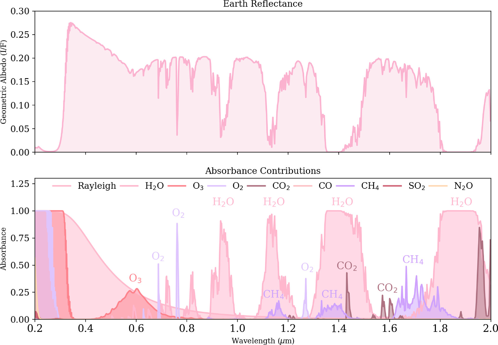
In this work, we use the spectral grid-based Bayesian inference method first described in N. Susemiehl et al. (2023, hereafter S23), and used in N. Latouf et al. (2023, hereafter BARBIE1) and N. Latouf et al. (2024, hereafter BARBIE2). In this method, 1.4 million geometric albedo spectra at discrete parameter values are generated, and forward models for Bayesian retrievals are then interpolated from the grid. However, the S23 grid has a limited wavelength range, operating primarily at optical wavelengths (0.5–1 μm), and consists of six varied parameters: surface pressure (P0), surface albedo (As), gravity (g), and H2O, O2, and O3 abundance. However, the limited set of atmospheric constituents bounded the applicability of the S23 grid to oxygen-rich atmospheric compositions at visible wavelengths (0.4–1.0 μm), and necessitated new grids to explore new wavelength ranges and atmospheric compositions. Figure 1 portrays a representative spectrum for an Earth twin in the top panel, and every molecule and their absorbance across the full spectral range of the new grids (0.2–2 μm) in the bottom panel. By focusing only on the visible, many molecular species are not considered, including key biosignatures such as CH4 and CO2. By building new grids with larger wavelength coverage and more parameters, we can further investigate the optimization of exoplanet characterization observations and build a more robust observing strategy for biosignatures.

Figure 1. In the top panel, we present a representative spectrum from our work where molecular contributions are visible, with the y-axis representing the geometric albedo. In the bottom panel, we present the absorbance contributions of every molecule available in the KEN grids, as well as the Rayleigh scattering also included: H2O, O2, O3, CH4, CO, CO2, SO2, and N2O, with the y-axis representing absorption. The x-axes are both the full wavelength range of the KEN grids (0.2–2 μm). Note that SO2 and N2O absorb at 0.2 μm very minimally, without features in other locations in this wavelength range.
Download figure:
Standard image High-resolution imageThis project is a direct continuation from BARBIE1 and BARBIE2, and in this paper we extend the same methodology to validate our new grids and study the impact of longer wavelengths (i.e., into the NIR) with CH4. In Section 2 we present the methodology of our grid building, validation, and simulations, also providing a brief summary of BARBIE1 and BARBIE2. In Section 3 we present the results of our simulations for modern and varying abundances of CH4, as well as an analysis of how CH4 and H2O detectability affect one another. In Section 4 we discuss the presented results and analyze the impact for future observations of varying Earth-twin epochs as a function of wavelength and further bandpass widths. In Section 5 we present our conclusions and ideas for future work.
2. Methodology
2.1. A New Grid-building Scheme
Although spectral retrieval studies have been used extensively to explore the detectability of atmospheric compositions for the direct imaging of exoplanets for multiple telescopes both current and future (e.g., R. E. Lupu et al. 2016; M. Nayak et al. 2017; A. J. R. W. Smith et al. 2020; M. Damiano & R. Hu 2022; A. V. Young et al. 2024), these retrievals are extremely computationally expensive. Most Bayesian retrievals use real-time radiative transfer calculations, combined with exploring large parameter spaces, mission capabilities, and constant model improvement that increase computation time to a rate that is not easily usable. Different methods to accelerate retrievals have been explored through efficient radiative transfer schemes or machine learning (e.g., P. Márquez-Neila et al. 2018; T. Zingales & I. P. Waldmann 2018; A. D. Cobb et al. 2019; C. Fisher et al. 2020; M. D. Himes et al. 2022; T. D. Robinson & A. Salvador 2023).
In order to facilitate the efficient production of new optimized spectral grids for our grid-based retrievals, we developed a Python package called Gridder, which is a generalized grid-building scheme based on the methodology of S23 (M. D. Himes et al. 2024, in preparation). Gridder produces arbitrary spectral grids using the Planetary Spectrum Generator (PSG), a publicly available radiative transfer model for creating planetary spectra (G. L. Villanueva et al. 2018, 2022). PSG can be used to calculate spectra over an ultrabroad wavelength range (50 nm–100 mm) and includes planetary atmospheres, surfaces, and bulk properties such as aerosols, atomic, continuum, and molecular scattering/radiative processes implemented layer by layer. The Gridder parameter structure is highly customizable, allowing any input parameter to PSG to be used as a parameter in the optimized grid, including parameterized thermal profiles (e.g., isothermal or adiabatic; M. R. Line 2013) and atmospheric chemistry (e.g., constant with altitude or thermochemical equilibrium). In addition to the error metric of S23, Gridder offers other common metrics, such as the maximum absolute percent error and mean squared error, for greater control over the resulting grid’s accuracy. Gridder features various optimizations (e.g., parallelization and checkpoints) to ensure efficient production of optimized spectral grids in a consistent, reproducible manner. Using Gridder, we have built a new set of spectral grids, each with six parameters to decrease the grid-building computational time, but over a far wider wavelength range from the UV to NIR (0.2–2.0 μm), and we have added the additional molecular atmospheric constituents CH4, CO2, CO, SO2, and N2O.
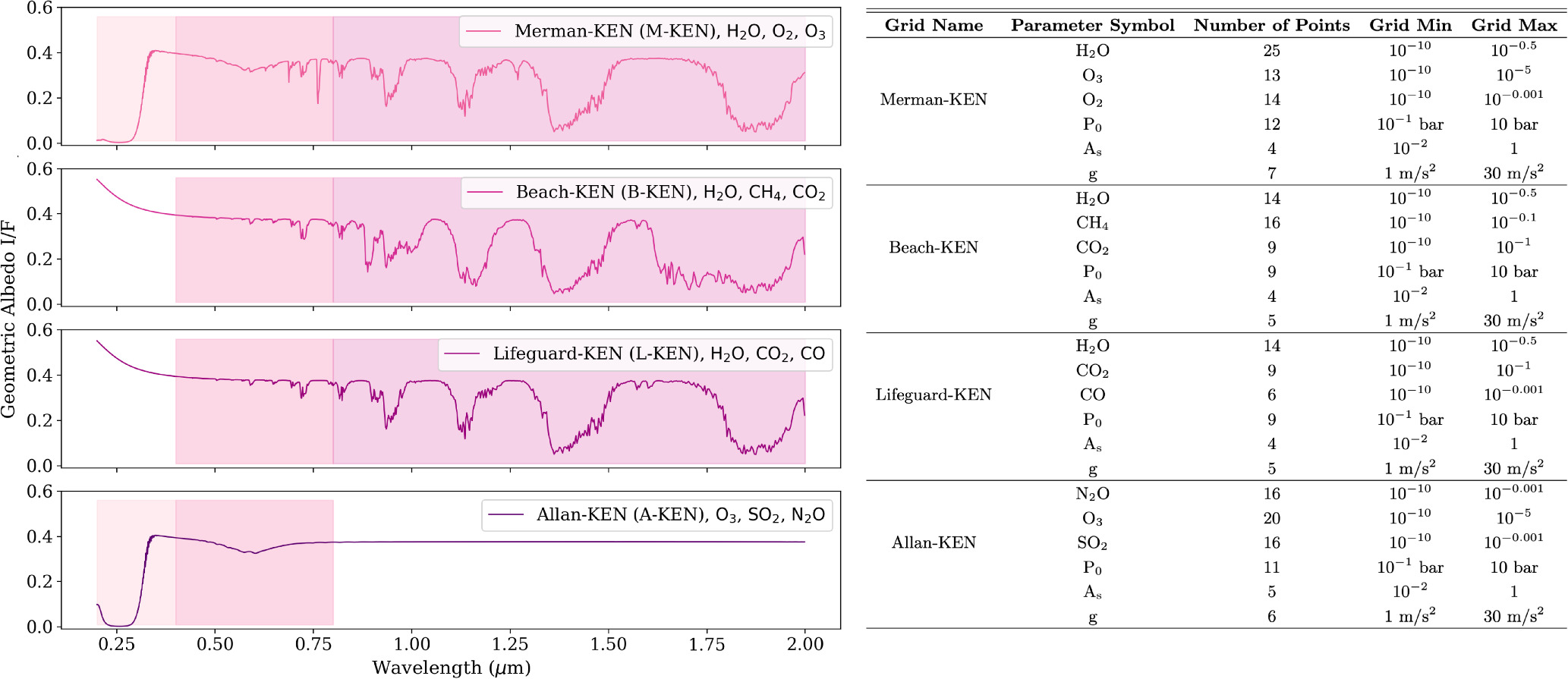
Our newly built grid set, hereafter the KEN grids (no acronym; they are just ken), allow for a direct comparison between grids since they cover the same wavelength range and the three base parameters of P0, As, and g with Rp fixed to 1 R⊕. However, they reduce the computational time by taking advantage of the different spectral regions covered by the absorption features of different molecules. Any molecules that have overlapping spectral features (for the range of atmospheric pressures examined) are housed within the same grid, while any that are orthogonal to each other do not need to be simultaneously retrieved within one grid, such as CH4 and O3. The background gas in each grid is set to N2 = 1 − P1 – P2 – P3 where P1 – P3 are the molecules per grid. In this way, we can also investigate the effects of false positive or negative molecular detection due to overlapping features. We developed four different spectral grids at a resolving power of 500 (R = 500), which can then be binned to lower resolving powers, with the ability to vary the cloud fraction Cf at any value between 0% cloudy to 100% cloudy. We describe the molecular parameters in each named grid in the KEN grid set, along with a modern-Earth-like spectrum per grid and the highlighted wavelength regimes for use per grid, in Figure 2.

Figure 2. Herein we present a modern, 50% cloudy, Earth-like spectrum for each grid over the full wavelength range, to illustrate the absence and presence of each molecule per grid. Each legend shows the name of the grid along with the present molecular constituents, with geometric albedo on the y-axis and wavelength on the x-axis. The highlighted regions portray the UV, visible, and NIR wavelength regions, and they are present in the grids that are most useful in said region. The table on the right contains the grid structure for all KEN grids (grid name, spacing, and number of points) for the clear grid versions. For the combined clear and cloudy grids, the overall size is doubled. It also includes the minimum and maximum values for each grid parameter.
Download figure:
Standard image High-resolution imageThe KEN grids will allow us to investigate varying atmospheric compositions beyond O2-dominated atmospheres, such as CH4 or CO2 dominated, to develop observational procedures for multiple planetary archetypes through wavelength.
2.2. BARBIE Methodology
We follow an identical methodological approach to that of BARBIE1 and BARBIE2 for the CH4 case study analysis. Herein we present a brief summary of the main steps in our analysis. For more detailed information, please see BARBIE1 and BARBIE2.
- 1.We set a modern-Earth twin as our fiducial data spectrum following Y. K. Feng et al. (2018), with isotropic volume mixing ratios (VMRs) of H2O = 3 × 10⁻³, O3 = 7 × 10⁻⁷, O2 = 0.21, constant temperature profile at 250 K, As of 0.3, P0 of 1 bar, and a planetary radius fixed at Rp = 1 R⊕. We bin our grid from the native resolving power of 500–140 and 70 for our simulations, and split the spectrum in 25 evenly spaced bandpasses across 20%, 30%, and 40% widths. R = 140 is generally accepted in the optical regime, while R = 70 is generally accepted in the NIR (The LUVOIR Team 2023). These ranges mimic the simultaneous bandpasses that may be achieved with high-performance coronagraphs in the future, or dual coronagraphs that can be used in combination (G. J. Ruane et al. 2015; E. H. Por 2020; R. Juanola-Parramon et al. 2022).
- 2.We run a series of Bayesian nested sampling retrievals using PSGnest10 housed in PSG. PSGnest is a Bayesian spectral retrieval methodology adapted from the original Fortran version of the Multinest retrieval algorithm (F. Feroz et al. 2009) and designed for application to exoplanetary observations (i.e., incorporating grid multidimensional interpolation, grid retrievals, the fitting methods, as well as the Multinest retrievals).
- 3.We receive the highest-likelihood values, the average values from the posterior distributions, uncertainties, and the log evidence (logZ; G. L. Villanueva et al. 2022) as outputs. We then calculate the log-Bayes factor (lnB; B. Benneke & S. Seager 2013); this compares retrievals with and without a given molecule to estimate the likelihood of the molecule’s presence in the exoplanet’s atmosphere. For our purposes, lnB < 2.5 is unconstrained (no detection), 2.5 ≤ lnB < 5.0 is a weak detection, and lnB ≥ 5.0 is a strong detection (see Table 2 of B. Benneke & S. Seager 2013). We also calculate the median and upper and lower limit values of the 68% credible region (J. Harrington et al. 2022). However lnB is a better estimation of detection rather than the 68% credible region since it is directly investigating the molecular presence versus absence and calculating which iteration yields the best fit, while the 68% credible region, by definition, includes the true value 68% of the time. lnB is not calculated for nongaseous components, since those factors cannot be absent.
This process is then repeated for varying abundances. For this work, we vary CH4 according to Table 1, following J. Kasting (2005) and L. Kaltenegger et al. (2007), while also adding values to bridge the large gap between abundance values (i.e., between Hadean and Archean values). The level of CH4 present in any specific habitable exoplanet atmosphere is uncertain, since CH4 production is significantly driven by biological activity; the same is true for any other biologically produced species. Since we are not running fully physically consistent chemistry models, we therefore use modern-Earth values as the default for other species as well as to isolate the effect of a single molecule, as in prior Bayesian Analysis for Remote Biosignature Identification on exoEarths (BARBIE) works. We also investigate the effects of H2O on CH4 detectability by testing a range of combined H2O and CH4 values, shown in Table 2. All retrievals were performed between 0.8 and 1.5 μm with 20%, 30%, and 40% bandpass widths, and R = 140 and R = 70. We carefully select a narrower wavelength range in order to investigate the detectability of CH4 in the optical or at the critical 0.9 μm H2O feature; this is currently poised as the first step in observations following the decision tree technique in A. V. Young et al. (2024).
Table 1. Values Used in Our Simulations for CH4
| CH4 (VMR) | Assumed Earth Epoch (Age) |
|---|---|
| 1.65 × 10⁻⁶ | Hadean (3.9 Gyr) |
| 1.65 × 10⁻³ | Archean (3.5 Gyr) |
| 7.07 × 10⁻³ | Archean (2.4 Gyr) |
| 1.65 × 10⁻³ | Proterozoic (2.0 Gyr) |
| 4.15 × 10⁻⁴ | Phanerozoic (0.8 Gyr) |
| 1.65 × 10⁻⁶a | Phanerozoic (0.3 Gyr)a |
Note. Moving from Earth-like values into different epochs of Earth’s history based on J. Kasting (2005) and L. Kaltenegger et al. (2007), and interpolating to provide more points between large gaps of abundance. aModern-Earth-like value.
Download table as: ASCIITypeset image
Table 2. All Values for CH4 and H2O Run for Our Analysis of Detectability Dependence on Molecular Abundance
| CH4 (VMR) | H2O (VMR) |
|---|---|
| 3 × 10⁻⁵ | 3 × 10⁻⁵ |
| 1 × 10⁻⁴ | 1 × 10⁻⁴ |
| 3 × 10⁻⁴ | 3 × 10⁻³ |
| 1 × 10⁻³ | 1 × 10⁻⁴ |
| 3 × 10⁻³ | 3 × 10⁻³ |
| 7 × 10⁻³ | 1 × 10⁻² |
Note. We tested all combinations of abundances, leading to 25 abundance combinations.
Download table as: ASCIITypeset image
3. Results
3.1. Grid Validation
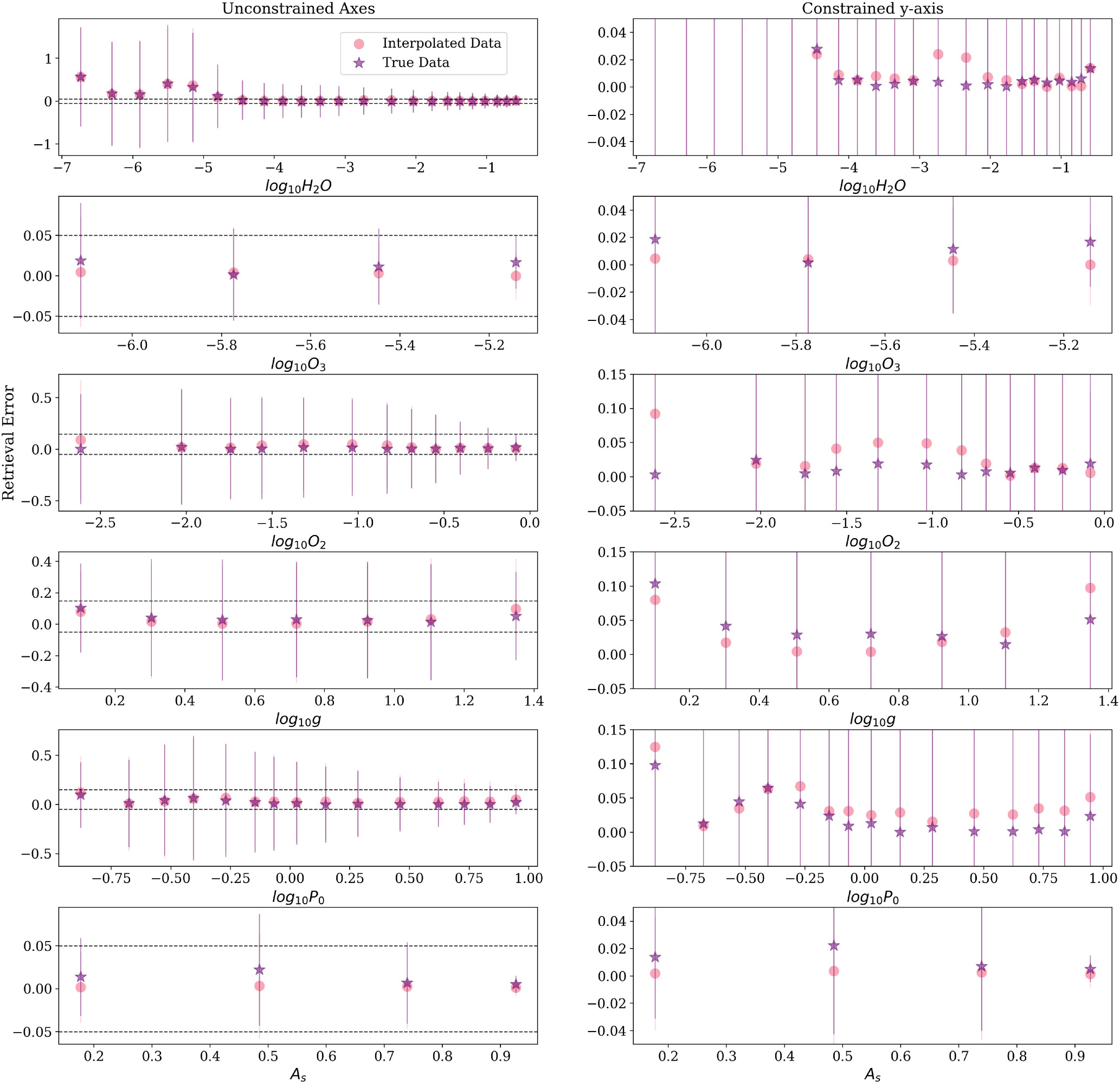
In S23 Figure 8, they investigate the interpolation error in the developed grid to ensure that the grid is not introducing a large error past any known interpolation error. We have replicated this in Figure 3 using the same technique as in S23 using our M-KEN grid, as that has the same parameters as in the S23 grid. To summarize, we ran 6D retrievals for each value of each parameter in the test grid. The test grid in use consists of the midpoint values of the M-KEN grid as the interpolation error is typically maximized near the midpoints, and thus to test the error we want to investigate the area of highest error. For each parameter set, a “true” spectrum was created (i.e., pulling the data spectrum directly from the midpoints grid) at an SNR of 20. The retrievals were then repeated, but the data spectrum was created by interpolating from the main M-KEN grid (i.e., the way that all retrievals will work when using KEN grids with PSGnest). We use the offset between the values retrieved for the “true” and interpolated spectra to assess the impact of interpolation error on these retrievals.

Figure 3. Interpolation error across a 6D retrieval across parameter space. The retrieval error is defined as the difference between the true and retrieved values. The pink dots represent retrievals performed on a spectrum interpolated from the KEN grid, and the purple stars represent retrievals performed on a PSG-calculated spectrum. The error bars on these points are drawn as the 68% credible regions. The left column shows the full y-axes, and the right column zooms in to the portion on the y-axes contained within the horizontal dashed black lines that cover the areas of lowest error.
Download figure:
Standard image High-resolution imageAlthough the M-KEN grid covers a wider wavelength range than the S23 grid, Figure 3 covers the wavelength range of 0.4–1 μm in order to directly replicate the range in S23. The error from retrieving on interpolated data is shown in pink dots, while the error from retrieving on “true” data is shown in purple stars. We also calculate the 68% credible region and portray those as error bars. The left column shows the full extent of the offset for every point, while the right column zooms in to the regions shown in the black dotted lines. We select these areas based on where there is a high concentration of overlapping points. Any differences between the results are due to an interpolation error.
We find that the retrieval error is generally very similar for both the “true” and interpolated data retrievals, with the derived retrieval error for both always within 1σ of the input value. The outlier errors, as in S23, are at small P0, and at large O3, although even those error ranges are no more than 15%. The average error hovers at below 5%, while the error between the interpolated and true data is never larger than 2% (with the singular exception of 10% at low O3). In fact, our error spread is much smaller than S23, validating that the new optimization procedures of Gridder yield higher fidelity results with a much faster overall runtime. This confirms that the Gridder selection of grid points has been successful, with the interpolation error not serving as a significant inhibitor for performing retrievals in this region.
To further isolate the impact of the retrieval error induced by interpolation within the grid apart from the Bayesian inference routine, we performed 4800 retrievals using the UltraNest package (J. Buchner 2016, 2019, 2021) on PSG-simulated spectra for values near the midpoints across the B-KEN grid’s parameter space. We use the grid’s native R = 500 spectral resolution and the full 0.2–2 μm wavelength range and assume an SNR of 15 for each wavelength channel. We find that the mean absolute error (MAE) between the maximum likelihood and the known true value is typically ∼0.02 for As and ∼0.2 for all other parameters when there is sufficient information content to constrain the parameter. This finding is generally consistent with Figure 3. When H2O, CH4, and CO2 can simultaneously be constrained, the MAE for the extrema of the 3σ region of all parameters is nearly equal to the MAE of the maximum likelihood, indicating that the 1D marginalized posteriors are offset from the known truth. This bias is generally negligible except in the case of g, where the mean absolute percentage error can be >60% at low values of  and ∼20% for Earth-like gravities. These results represent worst-case scenarios; under typical grid usage conditions (R = 140, reduced wavelength coverage, at least one parameter not at a grid midpoints), these errors will be reduced.
We present another analysis of grid efficacy in Figure 4, looking specifically at the deep CH4 feature centered at 1.1 μm. This presents modern-Earth values of all parameters except CH4, which is at an Archean value—increasing the CH4 value is necessary to investigate grid efficacy, as we expect it to be well constrained. This is using the B-KEN grid, which is also the grid used for all the science cases explored in this work. The B-KEN grid is the only KEN grid that contains CH4, thus it is our only option to investigate CH4 detectability. We find that there are no sharp cutoffs in our 1D histograms except for g, which can especially be seen in the 2D marginalized posterior for g and P0. However, g around the Earth value is the primary use case for these grids, which is well retrieved. CO2 and g also have significant posterior density at 1 × 10⁻¹⁰ VMR and 1 m s−2, respectively, indicating that the 68% credible region is underestimated. However, any molecule at such low abundances does effect spectral change, and CO2 is unconstrained in this wavelength region where there is no CO2. We also see known and expected degeneracies with As and Cf, with every parameter, especially the molecular parameters, heavily impacted, but every parameter is also retrieved within the 68% credible region.
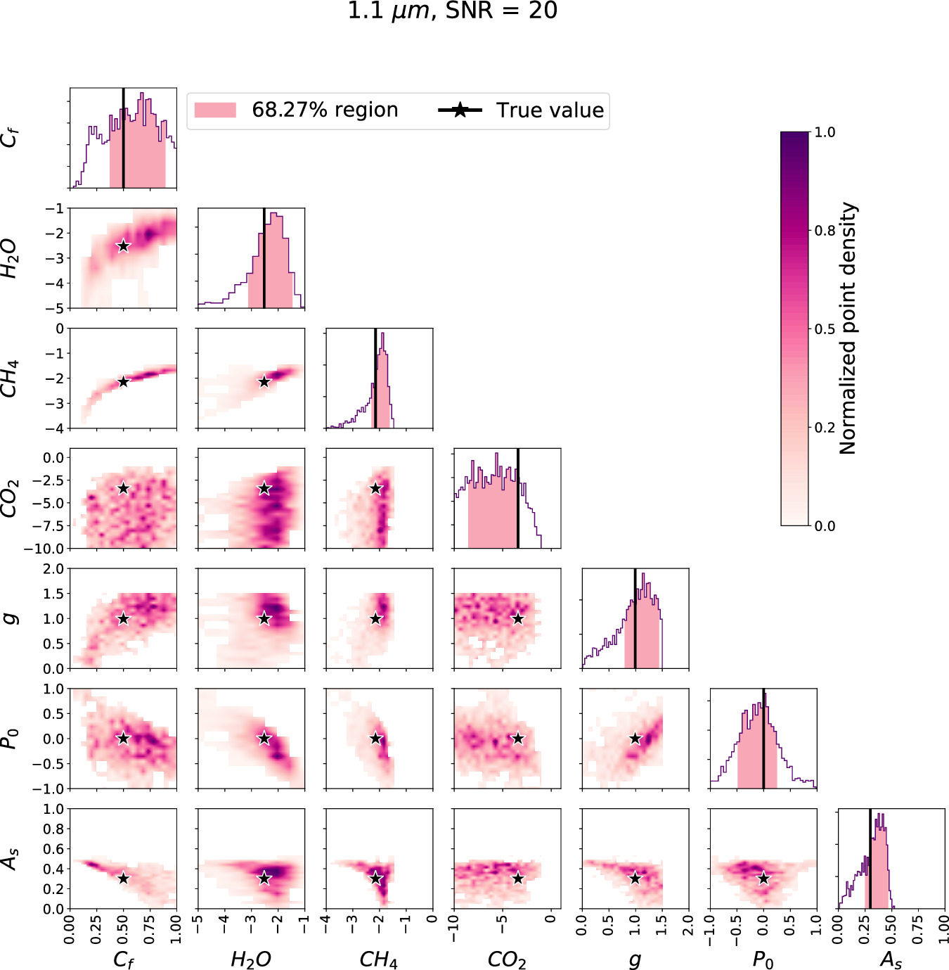
Figure 4. Corner plot for Archean CH4 abundance. The 68% credible regions are shown as pink shading in the 1D marginalized posterior distributions along the diagonal of the corner plot, and the true values are represented by black lines in the diagonals of the corner plot and black stars within the 2D plots.
Download figure:
Standard image High-resolution imageFor further analysis on grid, and Gridder, validation, please see M. D. Himes et al. (2024, in preparation) for a more thorough description.
3.2. Geologically Motivated CH4 Abundances
We begin by presenting the detectability of CH4 as a function of SNR for the fiducial modern-Earth case, as examined by S23, BARBIE1, and BARBIE2, to maintain consistency (all CH4 data and calculated lnB factors across abundance, SNR, and wavelength will be available to the community on Zenodo at doi:10.5281/zenodo.13760695). All other parameters were left to modern-Earth values, including a modern-Earth value of H2O. However, a modern level of CH4 (1.65 × 10⁻⁶) is completely undetectable at at all SNRs and bandpass widths tested at a resolving power of 140 and 70. Many other works have previously found the same result, due to the low concentration and thus weak absorption features (E. W. Schwieterman et al. 2018; M. Damiano & R. Hu 2022; S. Gilbert-Janizek et al. 2024; A. V. Young et al. 2024). Since a modern-Earth CH4 was not possible to detect, we quickly proceeded to the varying abundances listed in Table 1 to explore the minimum value at which CH4 could be detected.
For our abundance case study, we vary the abundance of CH4 above modern-Earth values up to a cap of the Archean-Earth value (7.07 × 10⁻³). We also vary the SNR for each abundance level to fully investigate the trade-off between higher SNR and molecular detectability. The CH4 abundances investigated are presented in Table 1, along with intermediate values to fill in the large gap between the Hadean and Archean epochs.
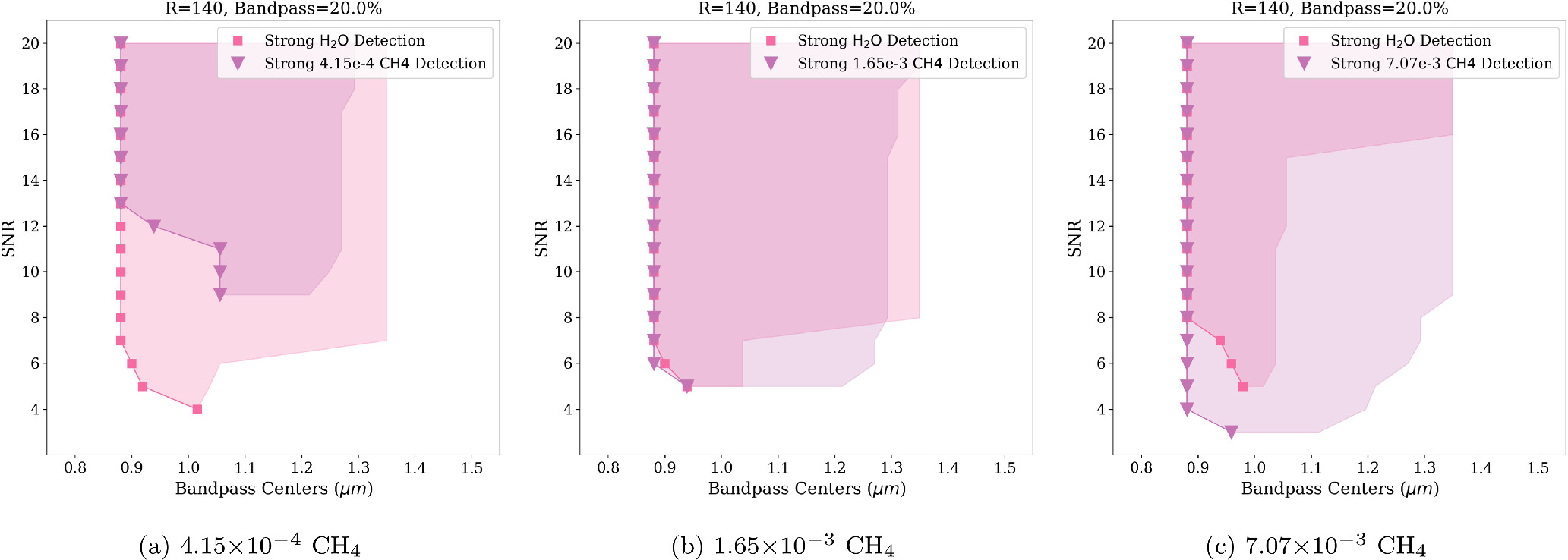
In Figures 5(a), (b), and (c), we present the strong detectability of the three highest CH4 abundances in our study, along with a modern H2O abundance for context, in purple triangles and pink squares, respectively. SNR is on the y-axis, with bandpass centers on the x-axis. We see that, as expected, as the abundance of CH4 increases, the required SNR for detection decreases, with SNRs of 9, 5, and 3 for CH4 abundances of 4.15 × 10⁻⁴, 1.65 × 10⁻³, and 7.07 × 10⁻³, respectively. Notably, at 4.15 × 10⁻⁴, the lowest SNR (9) is accessible at ∼1.05 μm, whereas at 1.65 × 10⁻³ and 7.07 × 10⁻³ abundances, the lowest SNRs are accessible at ∼0.9 μm. In order to achieve a detection of CH4 at 4.15 × 10⁻⁴ at 0.9 μm, an SNR of 13 is necessary.

Figure 5. Summary of the bandpasses where CH4 and H2O are detectable for 3 × 10⁻³ (modern) H2O and varying CH4 based on Table 1. The shortest bandpass center at which one can achieve a strong detection for H2O or a strong detection for CH4 are shown in pink squares and light purple triangles, respectively. SNR is on the y-axis, and the bandpass centers are on the x-axis. We also show the range out to the longest wavelength at which the same detection is achieved as shaded regions.
Download figure:
Standard image High-resolution imageLooking at the full range of abundance values in our study, we present a heat map showing detection strength as a function of SNR (y-axis) and CH4 abundance (x-axis) in Figure 6(a). The color bars represent the range of 0–5 lnB, between unconstrained and strong detection. We see here that CH4 is not strongly detectable until 4.15 × 10⁻⁴ (Phanerozoic), at which point an SNR of 9 is required. Moving to higher abundances significantly drops the required SNR for strong detection, with 1.65 × 10⁻³ (early Phanerozoic) requiring an SNR of 5 and 7.07 × 10⁻³ (Archean) detectable at all SNRs. At low abundances, such as a modern-Earth value of 1.65 × 10⁻⁶, CH4 is not detectable at any SNR. Interestingly, at 1 × 10⁻⁴ a weak detection is possible at an SNR of 20, with the next value of 4.15 × 10⁻⁴ only requiring an SNR of 9 for strong detection as mentioned, and an SNR of 6 for weak detection. This results in a very drastic change in CH4 detection over a relatively small change in abundance of CH4.
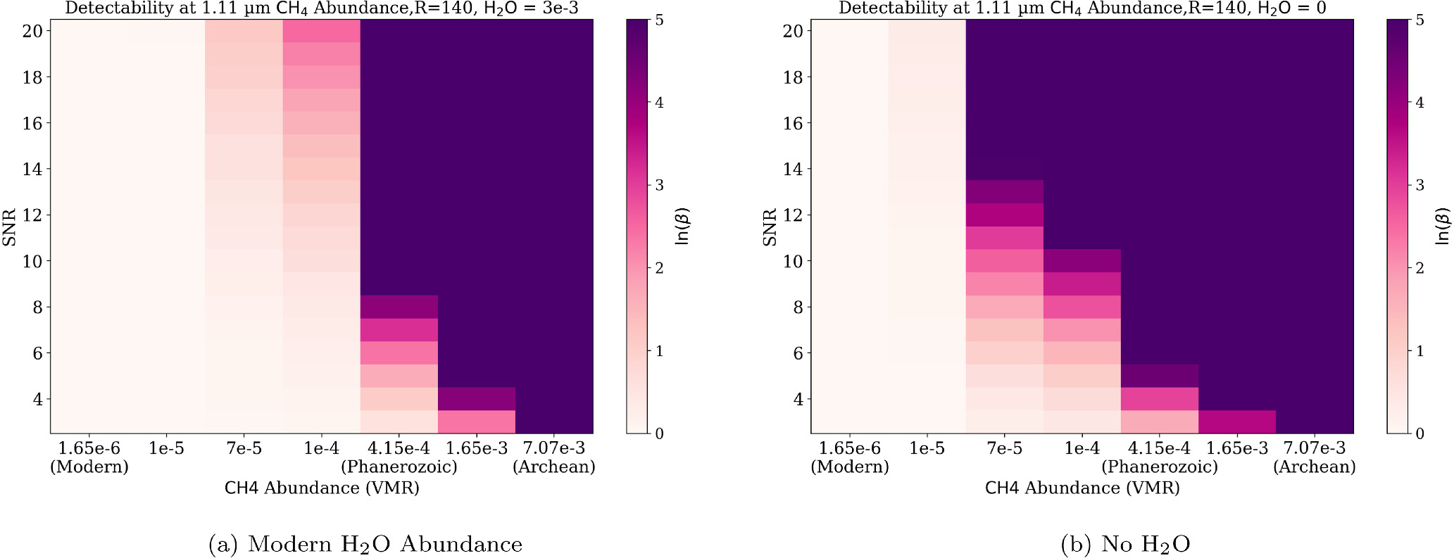
Figure 6. Heat map plots illustrating detection strength as a function of SNR and varying CH4 abundance with two H2O values. SNR is on the y-axis, CH4 abundance is on the x-axis, and the color bar shows the range of lnB from 0 to 5 to describe detection strength. lnB < 2.5 is unconstrained, 2.5 ≤ lnB < 5 is weak, and lnB > 5 is strong, as in prior figures.
Download figure:
Standard image High-resolution imageHowever, returning to Figure 5, we see a significant change in detectability for H2O across CH4 abundance. A higher SNR is required to detect H2O as CH4 increases. Also as the CH4 abundance increases, the range of strong H2O detection as a function of wavelength decreases, with a sharp cutoff at ∼1.1 μm. For wavelengths longer than 1.1 μm, it requires a high SNR (≥15) to detect H2O although there is a very large H2O feature at 1.35 μm. This indicates that the H2O features are being masked by strong CH4 features, thus H2O detectability is impacted.
This is confirmed in Figure 7, which presents a spectrum of modern H2O and three increasing values of CH4 in three panels (Phanerozoic and early and late Archean from top to bottom) as a function of wavelength and geometric albedo (x-axis and y-axis, respectively). As CH4 increases in abundance, the absorption feature aligns more closely with that of H2O, particularly between ∼1.1 μm and 1.2 μm. This results in an inflection point, wherein H2O is more difficult to detect due to the absorption feature being masked by the overpowering CH4. This led us to investigate the opposite effect—does H2O mask the detection of CH4 at lower CH4 abundance?
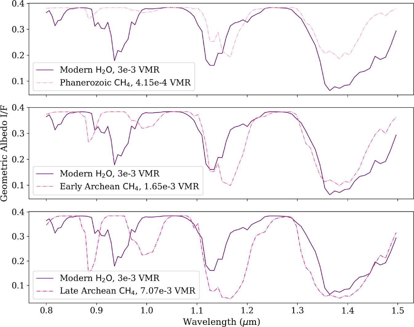
Figure 7. Multipanel plot illustrating overlap of H2O and CH4 features in the NIR wavelength regime. Wavelength is on the x-axis, geometric albedo (I/F) is on the y-axis. Each panel shows a modern level of H2O in dark purple, and a Phanerozoic, early Archean, and late-Archean abundances of CH4 in the top, middle, and bottom panels with a dotted–dashed line with a shade of pink, respectively.
Download figure:
Standard image High-resolution imageWe reran all values of CH4 in Table 1, however we set the abundance of H2O to zero in our fiducial spectrum. We find that, indeed, our detection of CH4 changes dramatically. In Figure 6(b), we again present a detectability heat map across all abundances of CH4 as in Figure 6(a), although with no H2O present. We see that CH4 is strongly detectable down to 7 × 10⁻⁵ VMR at an SNR of 14, and 4.15 × 10⁻⁴ VMR was detectable at an SNR of 6. Thus, with the absence of H2O, our detectable CH4 abundance shifts down over an order of magnitude. We can see the effect of H2O on CH4 detectability, and this can suggest that the abundance of CH4 cannot accurately be determined unless you also separately constrain the H2O abundance. However, we want to further understand the interactions between varying the abundances of H2O and CH4.
3.3. H2O and CH4 Detection Degeneracy
We ran a suite of retrievals with all combined H2O and CH4 values shown in Table 2, at 20%, 30%, and 40% bandpass widths—note that these values were selected purely to understand the inflection point of molecular abundance and detectability, with the highest H2O abundance at modern levels (3 × 10⁻³ VMR) and the highest CH4 abundance at Archean levels (7.07 × 10⁻³ VMR). Our lowest tested value of CH4 is (1 × 10⁻⁴ VMR), the first abundance at which any detection is possible.
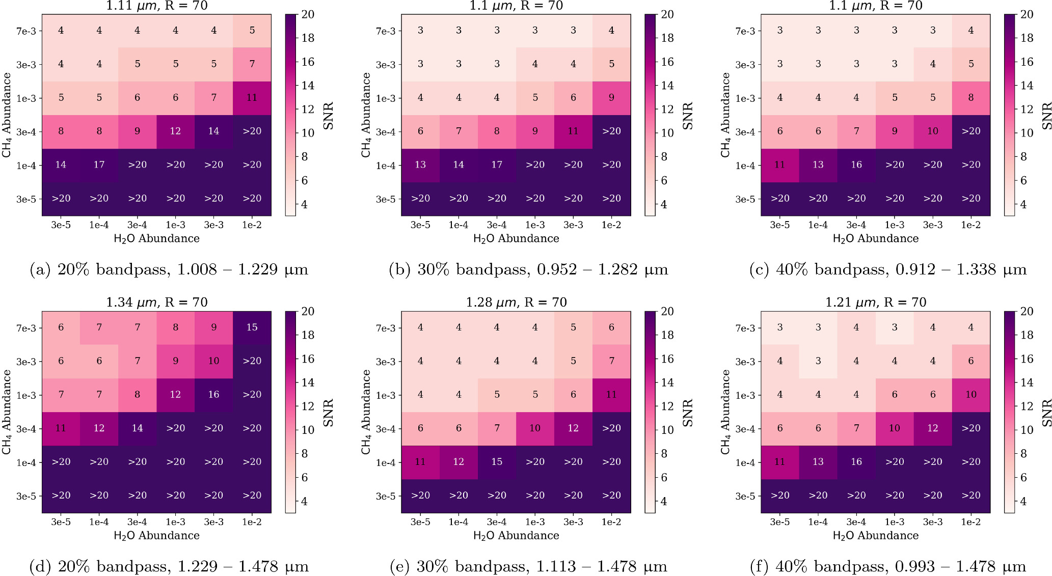
In Figure 8, we present the results of our degeneracy study as six heat maps at 1.1 μm and the longest possible bandpass (top and bottom rows, respectively), wherein the color corresponds to the SNR, with the required SNR for strong detection labeled on the plot. The x-axis is the H2O abundance, the y-axis is the CH4 abundance, with a 20%, 30%, and 40% bandpass width, respectively, in columns. All results are with R = 70, the current fiducial resolving power in the NIR. We can see as a trend in Figure 8 that the bandpass width has a very large impact on detectability for CH4 as a function of abundance: at high CH4 abundances, especially at 1.1 μm where there is a large CH4 absorption feature, the Archean levels of CH4 remain essentially unchanged through bandpass width. This reaffirms our earlier results that high CH4 did not vary through bandpass width and that H2O abundance is a large factor in detectability. Looking first to Figures 8(a)–(c), at high CH4 values, 3 × 10⁻³ VMR and above, the H2O abundance minimally influences the CH4 detectability. We begin to see an influence in detectability at 1 × 10⁻³ VMR, where at the lowest H2O abundance (3 × 10⁻⁵ VMR) the required SNR for CH4 detection is ∼4, through the central H2O abundances, the required SNR is ∼6 for CH4 detection, and at the highest H2O abundance (1 × 10⁻² VMR), the required SNR for CH4 detection is up to 11 at a 20% bandpass, and an 8 for a 40% bandpass. The CH4 abundance is unchanging across this range of H2O abundances; thus it is clear that the influence must be H2O. This influence continues to grow stronger as the CH4 abundance decreases, with 3 × 10⁻⁴ VMR CH4 abundance requiring an SNR of 8 at the lowest H2O abundances for a 20% bandpass and 6 for 30% and 40%, and an SNR higher than 20 (i.e., undetectable in our study) at the highest H2O abundances. The degeneracy is most obvious at 1 × 10⁻⁴ VMR CH4 abundance, with each increasing abundance of H2O increasing the required SNR for strong CH4 detection—and resulting in no detections.

Figure 8. SNRs for strong CH4 detection. Heat maps of CH4 detectability as a function of molecular abundance for R = 70, at 1.11 μm (top row) and centered on the 1.3 μm feature (bottom row). We present 20%, 30%, and 40% bandpass widths. y-axis: CH4 abundance, x-axis: H2O abundance, and heat: SNR. Required SNRs for strong detection are written on the associated block, unless there is no strong detection, thus labeled “>20.”
Download figure:
Standard image High-resolution imageIn Figures 8(d)–(f), we adjust the wavelength that is being investigated. Since the bandpass centers change as the bandpass width increases, the final bandpass is investigated in Figures 8(d)–(f) with different bandpass centers. The emphasis in this last bandpass is in the 1.3 μm feature that appears for both CH4 and H2O. We find a similar trend to the above, with higher SNR requirements at each bandpass. With the 20% bandpass width (Figure 8(d)) specifically, the required SNR is higher than in Figures 8(a)–(c), especially at high H2O. In fact, at the highest value of H2O (1 × 10⁻² VMR), CH4 is not detectable at 3 × 10⁻³ VMR and 1 × 10⁻³ VMR although both of those abundances were still detectable at shorter wavelengths. Thus longer wavelengths (e.g., 1.35 μm) are not well suited for CH4 detection, especially with narrower bandpasses.
Next, we investigate H2O detectability. We present in Figure 9 another set of heat maps to investigate how the detection of H2O changes as a function of CH4 abundance. All plot aspects remain the same as Figure 8, with the exception that we are investigating H2O detectability. We again see that there is a strong correlation with the bandpass width, with detectability increasing as the bandpass width increases, especially at shorter wavelengths. At shorter wavelengths, such as 1.1 μm, H2O is detectable at all but the lowest abundances, with changing SNR. At a modern-Earth level of H2O, detectability at a 20% bandpass width requires at most an SNR of 12 and more than halves to an SNR ≤ 5 for a bandpass width of 40%. However, this does not hold for long wavelengths. We find that at longer wavelengths, the high CH4 abundances completely mask the H2O features leading to an inability to detect H2O at high CH4 or low H2O. However, we did find that at low H2O and sufficiently low CH4, the presence of both molecules together increases the detectability of H2O, likely due to the degeneracy between the two molecules being broken in this wavelength regime.
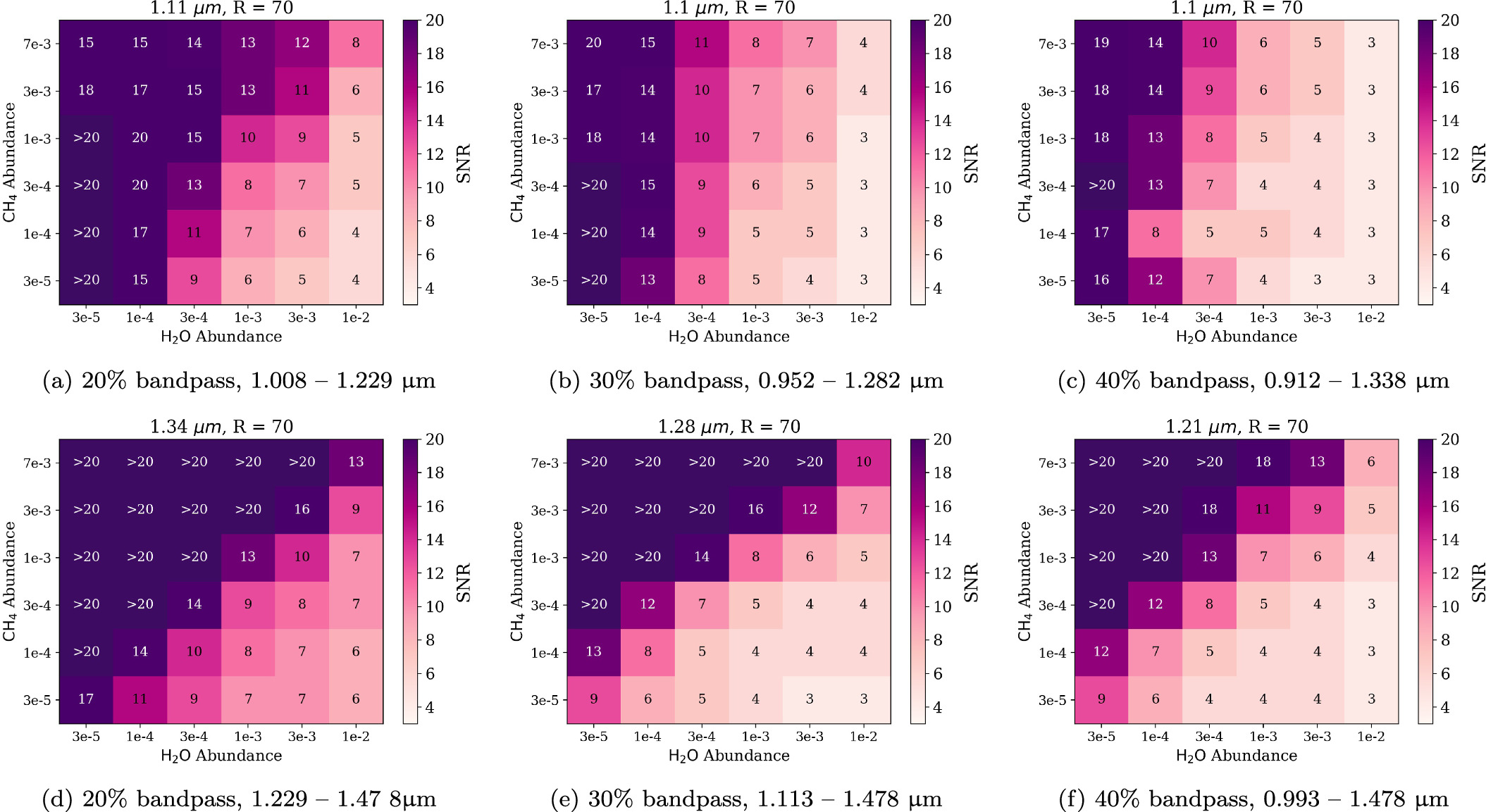
Figure 9. SNRs for strong H2O detection. All plot facets remain the same as Figure 8, but illustrating H2O detectability.
Download figure:
Standard image High-resolution image4. Discussion
Understanding the potential for dual detection of atmospheric constituents is an important factor in optimizing the required telescope observing time. Figure 5(a) shows how crucial this investigation is in the NIR. At the lowest detectable values of CH4 in our initial investigation, in order to detect both H2O and CH4 an SNR of 9 is required at 1.1 μm, and this remains possible out to 1.2 μm. In order to detect both H2O and low CH4 at shorter wavelengths, such as at 0.9 μm, an SNR of ≥13 is required. This is a significant difference in SNR and would result in a drastic increase in the required exposure time. However, the optimal wavelength for a detection of both molecules reverses at higher CH4 abundances—the detectability of H2O is impacted at longer wavelengths as shown in Figure 5(c). In order to detect both H2O and CH4 at 1.1 μm, an SNR of ≥15 is required; however, at 0.9 μm the combined detection is accessible at an SNR of 5. We begin to see that there is a relationship between H2O and CH4, which is further confirmed by the degeneracy between H2O and CH4 shown in Figure 4.
The overlap of molecular absorption features as shown in Figure 7 drives this degeneracy. The bottom most panel shows both a modern-Earth H2O abundance (3 × 10⁻³ VMR) and a late-Archean-Earth CH4 abundance (7.07 × 10⁻³ VMR). At 0.9 μm, we can see the absorption features are orthogonal to each other and thus more easily disentangled. At 1.1 μm and longer, the CH4 feature absorbs much deeper and wider than the H2O feature, thus completely preventing the possibility of detection without a high SNR. The opposite effect is seen at lower CH4 abundance, such as the Phanerozoic abundance (4.15 × 10⁻⁴ VMR) shown in the top panel of Figure 7. Here, the CH4 features at 0.9 μm are too shallow to be detected without high SNR, and at longer wavelengths (such as 1.4 μm), the CH4 feature is completely contained within a much larger H2O feature and is thus not detectable. At 1.1 μm, both CH4 and H2O are detectable due to the slight offset between the absorption features. We can clearly see that the detectability is a function of the abundance of CH4 and H2O, and the abundances of CH4 and H2O are degenerate in certain regimes.
To further investigate this degeneracy, we first looked at comparing a null versus modern H2O value in Figure 6, specifically at 1.1 μm where the overlapping features compete. In Figure 6(a) with modern-Earth H2O abundance, we achieve a strong CH4 detection at 4.15 × 10⁻⁴ VMR at SNR = 9, while still achieving at most a weak detection at 1 × 10⁻⁴. Comparatively, in Figure 6(b) 4.15 × 10⁻⁴ VMR requires an SNR of 6 for strong detection with no H2O present, compared to the previous SNR of 9. This confirms that H2O are degenerate, with detectability reliant on the abundances, and thus we explored a range of abundance values of H2O and CH4 to finely understand the relationship we found.
In Figures 8 and 9, we see that there are clear degeneracies between H2O and CH4, but with further varying relationships through wavelength. We find that the detectabilities of H2O and CH4 are both a function of CH4 and H2O abundances, wavelength, and bandpass width. In Figures 8(a)–(c) and 9(a)–(c), we can clearly see that both molecules are far easier to detect, at all bandpass widths, in this wavelength regime when comparing to Figures 8(d)–(f) and 9(d)–(f) presenting CH4 and H2O at longer wavelengths. At longer wavelengths, both molecules are more difficult to detect, with more abundance values undetectable. Critically, a modern-Earth level of H2O is detectable at all CH4 abundances and bandpass widths at 1.1 μm while it is undetectable at 20% and 30% bandpasses at Archean levels of CH4 at 1.3 μm. Similarly, CH4 is more accessibly detectable across bandwidth at shorter wavelengths, and detectability worsens across the board at longer wavelengths. With this, we can dismiss the possibility of looking for CH4 and H2O at the longer wavelengths considered in this study (e.g., 1.35–1.5 μm).
Focusing on the shorter, 1.1 μm wavelength (i.e., Figures 8(a)–(c)), we see a steady trend of increased SNR requirements for CH4 abundances as a function of H2O abundance. At the Archean abundance, which is of high interest, we see that there is essentially no impact to the CH4 SNR requirements. However at lower values that can be used as guides for other epochs, such as 3 × 10⁻⁴ VMR for the Phanerozoic epoch, we see changes in the required SNR for CH4 detection. At the lowest H2O abundance an SNR of 8 is required at a 20% bandpass width, while at the modern H2O abundance (3 × 10⁻³ VMR) an SNR of 10 is required—thus the required SNR for detection almost doubles across the H2O abundance ranges, becoming undetectable at higher H2O abundances. When moving to lower abundances of CH4 this effect is more pronounced, requiring higher base SNRs at the lowest H2O abundance and becoming undetectable at mid to high H2O abundances. This is especially crucial when we consider that, although a modern-Earth abundance of CH4 (1.65 × 10⁻⁶ VMR) is not detectable, a high H2O abundance can mask the detection of CH4 at low to mid-level values.
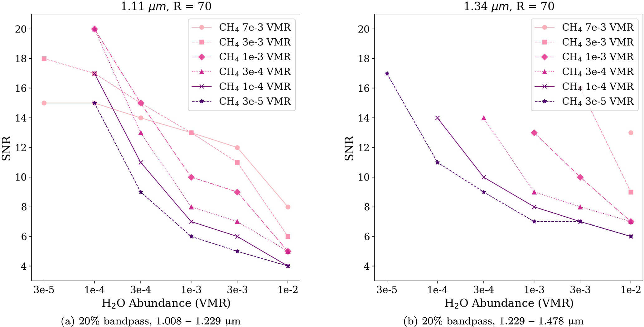
Figure 10 shows the CH4 and H2O degeneracy in more detail. We present the minimum SNR required per H2O abundance for H2O detectability at each CH4 abundance at R = 70 and two wavelengths: 1.1 μm in Figure 10(a) and 1.34 μm in Figure 10(b). In Figure 10(a) we can see that, as before, 3 × 10⁻⁵ VMR H2O is only accessible at the two highest values of CH4 at 1.1 μm, while otherwise the lowest detectable H2O abundance is 1 × 10⁻⁴ VMR at all other CH4 values. When moving to longer wavelengths in Figure 10(b), the low abundances of H2O are only accessible at the lowest CH4 abundances, due to the dual molecular features breaking the spectral degeneracy.
Figure 10. SNRs for strong H2O detection. Plot of the lowest SNR values at which a strong detection is achieved for all H2O values in our degeneracy investigation at (a) 1.1 μm and (b) 1.34 μm with a 20% bandpass at R = 70. The H2O VMR values are on the x-axis, with SNR on the y-axis. Each line represents a different tested CH4 value in VMR, labeled in the figure with different line styles and markers.
Download figure:
Standard image High-resolution image
Additionally, although shorter wavelengths are clearly preferred for dual CH4 and H2O detection, the 0.9–1.1 μm regime is burdened with increased coronagraph detector noise as detailed below, leading to longer required exposure times and thus higher required SNRs for detection.
5. Conclusions and Future Work
To summarize, we find the following points.
- 1.Modern levels of CH4 (1.65 × 10⁻⁶ VMR) are not detectable at any SNR ≤ 20 with any bandpass width. Archean levels of CH4 (7.07 × 10⁻³ VMR) are easily detectable at all SNRs and bandpass widths.
- 2.CH4 detectability is a function of the abundances of both CH4 and H2O, due to the close overlap of spectral features for both species. This overlap between CH4 and H2O absorption features becomes most acute at low to moderate CH4 abundances, and as the H2O abundance increases, the required SNR for CH4 detection increases.
- 3.H2O detectability depends on the abundance of CH4; as CH4 abundance increases, the required SNR to detect low to moderate H2O increases.
CH4 and H2O detectability clearly relies heavily on the bandpass selected for observation. At longer wavelengths, detectability drops for both molecules, and instrument efficiency decreases as a result of moving further into the NIR. Shorter wavelengths remain preferable for detection, namely at 1.1 μm for both CH4 and H2O, and 0.9 μm for H2O. However, when searching for moderate to low CH4 in an H2O-rich atmosphere, or searching for moderate to low H2O in a CH4-rich atmosphere, a higher SNR will be required to disentangle the molecular absorption signals. This may impact the science goals for HWO depending on whether an Archean-Earth atmosphere or a modern-Earth atmosphere drives the SNR requirement.
In future works, the BARBIE project will culminate with an investigation of molecular detection across the full expected wavelength range for the HWO. We will explore the requirements for molecular detection across the UV, optical, and NIR to determine the optimal wavelength range and SNR per molecule for strong detection. These metrics will be coupled with also varying the bandpass width across 20%, 30%, and 40% bandpasses, with the new addition of a 10% bandpass width. By using the KEN grids, we will explore molecular relationships through wavelength to investigate the most efficient observing strategy to detect multiple molecules with the most optimal bandpass wavelength, width, and SNR.
We also note that many of the critical wavelength bandpasses for optimal observation of H2O fall at the intersection of the high-sensitivity regions of different detector technologies. This wavelength dependency could significantly impact the requirements for biosignature detection and result in significant differences to characterization yields, as shown by C. C. Stark et al. (2024). In future works, we will investigate how coronagraph detectors and their wavelength-dependent sensitivity can vary the detectability of different molecular species.
Acknowledgments
N.L. gratefully acknowledges financial support from an NSF GRFP and NASA FINESST. N.L. gratefully acknowledges Dr. Joseph Weingartner for his support and editing. N.L. also gratefully acknowledges Greta Gerwig, Margot Robbie, Ryan Gosling, Emma Mackey, and Mattel Inc.TM for Barbie (doll, movie, and concept), for which this project is named after. This Barbie is an astrophysicist! The authors would like to thank the Sellers Exoplanet Environments Collaboration (SEEC) and ExoSpec teams at NASA’s Goddard Space Flight Center for their consistent support. M.D.H. was supported in part by an appointment to the NASA Postdoctoral Program at the NASA Goddard Space Flight Center, administered by Oak Ridge Associated Universities under contract with NASA.