

Disconnectivity matters: the outsized role of small ephemeral wetlands in landscape-scale nutrient retention
Published 24 January 2023 •
© 2023 The Author(s). Published by IOP Publishing Ltd
,
,
Citation Frederick Y Cheng et al 2023 Environ. Res. Lett. 18 024018DOI 10.1088/1748-9326/acab17
You need an eReader or compatible software to experience the benefits of the ePub3 file format.
Article metrics
6075 Total downloads
0 Video abstract views
Submit
Submit to this JournalDates
- Received 30 August 2022
- Accepted 13 December 2022
- Published 24 January 2023

Peer review information
Method: Double Anonymous
Revisions: 1
Screened for originality? Yes
Abstract
Wetlands protect downstream waters by filtering excess nitrogen (N) generated from agricultural and urban activities. Many small ephemeral wetlands, also known as geographically isolated wetlands (GIWs), are hotspots of N retention but have received fewer legal protections due to their apparent isolation from jurisdictional waters. Here, we hypothesize that the isolation of the GIWs make them more efficient N filters, especially when considering transient hydrologic dynamics. We use a reduced complexity model with 30 years of remotely sensed monthly wetland inundation levels in 3700 GIWs across eight wetlandscapes in the US to show how consideration of transient hydrologic dynamics can increase N retention estimates by up to 130%, with greater retention magnification for the smaller wetlands. This effect is more pronounced in semi-arid systems such as the prairies in North Dakota, where transient assumptions lead to 1.8 times more retention, compared to humid landscapes like the North Carolina Pocosins where transient assumptions only lead to 1.4 times more retention. Our results highlight how GIWs have an outsized role in retaining nutrients, and this service is enhanced due to their hydrologic disconnectivity which must be protected to maintain the integrity of downstream waters.

Original content from this work may be used under the terms of the Creative Commons Attribution 4.0 license. Any further distribution of this work must maintain attribution to the author(s) and the title of the work, journal citation and DOI.
1. Introduction
Wetland protection and restoration has been recognized as one of the most promising strategies for mitigating nutrient pollution [1–3]. Wetlands retain excess nutrients from agricultural and urban runoff and protect downstream waters [4–6]. In particular, the anoxic conditions and high organic carbon content in wetlands promotes the removal of nitrogen (N) through denitrification [7]. Indeed, wetlands in the United States have been estimated to remove more reactive N than all other aquatic ecosystems combined, in addition to providing other ecosystem services such as carbon sequestration and biodiversity enhancement [8–11].
Prioritization of wetland restoration requires an understanding of how different types of wetlands across the landscape perform different services [12]. The effectiveness of N retention in a wetland varies widely, with retention magnitudes ranging from 0.002 to 9048 g N m−2 yr−1 and retention efficiencies ranging between 30% and 40% of N inputs [6, 13, 14]. Retention rates have been found to correlate strongly with inputs from the landscape, wetland size, and water residence times [6, 15, 16]. At the landscape-scale, N retention potential of wetlandscapes can be quantified as a function of N retention in individual wetlands, as well as the distribution and connectivity of wetlands across the landscape. Hansen et al used a coupled model to explore N retention dynamics in the Le Sueur River Basin in the Minnesota River basin, and found restoration of floodplain wetlands to be the most cost-effective strategy for N retention [17]. Evenson et al found that restoring 2% of the area of the Upper Mississippi River Basin to wetlands can reduce the outlet N loads by 12% [18]. Cheng et al estimated N removal in over 30 million wetlands across the contiguous US, and found that a targeted 10% increase of current wetland area in zones of the highest nitrogen inputs can reduce N loads to the Gulf of Mexico by 40% [10].
An important class of wetlands is geographically isolated wetlands (GIWs), defined as wetlands that are completely surrounded by uplands, lack a persistent surface water connection to navigable streams, and may contain water for only part of the year [19]. GIWs span many wetland types and hydrogeomorphic settings (e.g. prairie potholes in Midwestern US and Central Canada, vernal pools of New England and eastern Canada, Delmarva and Carolina Bays, playas of southwestern US and Mexico,), and have traditionally received less protection due to their apparent disconnectivity from downstream navigable waters [20, 21]. They are also generally smaller than most riparian wetlands and contain water for only a part of the year [12]. GIWs typically receive seasonal water inputs through snowmelt or intense storms and lose water in subsequent months through evapotranspiration or groundwater recharge [19, 22]. From a biogeochemical perspective, GIWs often receive the first flush of solutes from the landscape [23] and the lack of direct connection to the river network increases processing times and nutrient retention, making them landscape biogeochemical hotspots [5, 24]. Also, while the lack of apparent connection to surface waters increases their ability to be most effective as nutrient filters, it is this lack of connection that excludes them from the Clean Water Act and makes them most vulnerable to loss [5, 21].
The nutrient retention potential of GIWs is a function of their inundation characteristics that drives water residence times and reaction dynamics [6]; yet most studies on wetland N retention at large scales focus on a fixed wetland area derived from national scale wetland inventories, and have not incorporated spatially explicit, sub-annual inundation information. There is currently a lack of quantitative understanding of the temporal dynamics of water storage in small ephemeral GIWs, and how such dynamics can potentially affect their nutrient retention potential. In a recent paper, Park et al used 30 years of satellite imagery to explore the seasonal dynamics of water storage in ten wetland regions across the US [25]. Our objective is to build on this work and explore the linkages between water storage and nutrient retention dynamics. Specifically, we focus on the following questions: (a) what is the role of inundation dynamics on nutrient retention in wetlands? (b) How does the inundation-retention relationship vary as a function of wetland size? (c) How does wetland size and climate interact to alter these relationships for different wetlandscapes?
2. Methods
2.1. Wetland inundation and bathymetry data
We modeled N retention dynamics in eight wetland regions of the continental US representing different climate and geomorphology: California vernal pools, prairie potholes in North Dakota, basin wetlands in Minnesota, cypress domes in Florida, Texas playa lakes, North Carolina pocosins, coastal plain wetlands in Georgia, and Nebraska sandhills. Within each of these eight landscapes, a 1000 km2 rectangular region was selected based on the presence of a high density of National Wetlands Inventory (NWI) wetlands, and infrequent gaps in remote sensing data [25]. GIWs were then derived within the selected rectangular regions using the NWI and National Hydrography Dataset (NHD), following the methodology outlined in Park et al [25]. Briefly, the method involves filtering the NWI dataset to focus only on palustrine and lacustrine wetlands. First, the NHD was used to create 10 m buffer polygons to filter out rivers, lakes >8 ha, other water bodies >1.5 ha, other flowlines or features, and all palustrine and lacustrine wetlands within the 10 m NHD buffered polygons were removed. Bathymetric relationships for each GIW were then derived to convert observed inundated areas to volume estimates. This was determined using the 1/3rd arc-second USGS DEM [26] cropped to the GIW extent, and starting from the top of the wetland incrementally determining the areas and volumes at each vertical increment using the rasterio python package [27].
We then characterized the inundation dynamics of the GIWs using the global surface water (GSW) dataset that was derived from Landsat imagery and contains monthly observations of surface water body extent [28]. By intersecting the boundaries of the identified GIWs with the GSW dataset, we developed a monthly time series of wetland inundated areas and volumes between 1985 and 2015. The method led to the characterization of 3698 GIWs across the eight wetlandscapes, with the greatest density of GIWs in the 1000 km2 block in North Dakota, and much fewer GIWs in the vernal pools and the North Carolina pocosins (table 1). We treat each year of data for each wetland separately in the subsequent analysis, and refer to each as a wetland-year. Use of the remotely sensed observed inundation data allows us to integrate climate (e.g. dry and wet years) and landscape factors (e.g. downstream and upland wetlands), as well as various human controls (managed and unmanaged wetland systems) that contribute to the inundation dynamics.
Table 1. Summary of GIWs and wetlandscape characteristics used in analysis.
| State | Wetland type | Aridity index (AI = PET/P) | Number of GIWs identified | Total wetland-years of record | Median log (Area in m2) (interquartile range) |
|---|---|---|---|---|---|
| CA | Vernal pools | 2.90 | 27 | 392 | 3.43 (3.25–3.86) |
| FL | Cypress domes | 1.33 | 250 | 1287 | 3.73 (3.25–4.23) |
| GA | Coastal plain | 1.26 | 35 | 392 | 3.55 (2.95–4.18) |
| MN | Basin wetlands | 1.21 | 48 | 54 | 3.43 (2.95–3.56) |
| NC | Pocosins | 1.23 | 27 | 504 | 3.73 (3.25–4.13) |
| ND | Prairie potholes | 2.31 | 2395 | 12 570 | 3.65 (3.25–4.16) |
| NE | Sandhills | 3.17 | 864 | 574 | 3.43 (2.95–3.86) |
| TX | Playa lakes | 4.71 | 52 | 589 | 4.61 (3.80–5.03) |
2.2. Transient wetland N retention dynamics
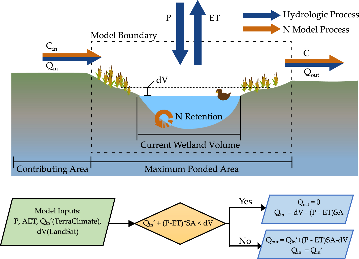
A reduced-complexity model was developed to estimate temporal fluctuations in N retention dynamics in a wetland as a function of time-varying inflows and outflows (figure 1). Assuming well-mixed conditions within the wetland, the rate of change of nitrogen mass M [M] within the wetland was described as:
where Qin is the volumetric flux of water entering the wetland from its contributing area [L3/T], Cin is the N concentration in the water entering the wetland [M/L3], Qout is the volumetric flux of water leaving the wetland as recharge or surface outflow [L3/T], V is the ponded wetland volume [L3], and k is a first order N retention rate constant [T−1] that describes the temporary (e.g. plant uptake, burial) and permanent (e.g. denitrification) processes that contribute to N retention in wetlands. While further differentiation of the surface and groundwater pathways of water and nitrogen could provide additional insight on how wetlands behave, there is insufficient data to quantify how the flows and solutes are partitioned. As our study aims to quantify the within-wetland dynamics, this model structure can still address how nitrogen retention is affected by downstream disconnectivity.
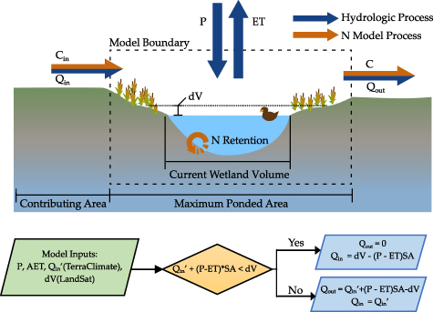
Figure 1. Conceptual model framework. Wetland schematic showing fluxes and stores, and algorithmic flow chart for the reduced complexity hydrology model.
Download figure:
Standard image High-resolution imageWe estimated k (d−1) using an empirical relationship developed by Cheng and Basu [6], that used measured N flux data, as well as water flow and surface area information (SA; m2) from 178 wetlands across the world:

The inverse relationship was attributed to the higher ratio of reactive sediment area to water volume in smaller wetlands that increases the opportunity for N in the water column to come in contact with the sediments, where N is removed by denitrification. Of course, other factors such as temperature and soil redox conditions that are specific to the different regions will impact the k values; however, Cheng and Basu’s meta-analysis highlights that wetland morphology acts as one of the most important first-order controls [6]. This simplification allows us to estimate k values at regional scales using wetland SA data that is easily accessible. Cheng et al used this relationship to estimate wetland N removal in 30 million wetlands across the continental US [10]. However, they assumed wetland area to be invariant in time. As a small wetland dries up over the course of a season, the reactive SA to volume ratio increases, and this can increase the retention rate constant even further. Here, we use time-varying SA of the wetlands from remotely sensed data to estimate time-varying k using equation (2).
Remotely sensed wetland inundation data was also used to estimate the time-varying wetland volumes, as well as inflows and outflows Qin and Qout from the wetland. Specifically, we used estimated monthly ponded volumes of the wetland (V), and available data for rainfall, evapotranspiration and runoff to estimate the inflows and outflows with the following mass balance [29]:
where P is the direct precipitation rate on the wetland [L/T], ET is the evapotranspiration rate from the wetland surface [L/T], and SAmax is the maximum inundated SA of the wetland over the 30 years of available remote sensing data [L2]. Although the ponded area of the wetland changes over time, we assumed direct precipitation to be intercepted by the maximum area. Additionally, though direct ET occurs only from the inundated area, we used the maximum SA to estimate the overall ET flux, given ET in the moist margins of the wetland can induce losses from the ponded area through local groundwater exchange [30].
Monthly precipitation (P), evapotranspiration (ET) and runoff (Q) from the TerraClimate dataset [31] was used to estimate Qin and Qout (figure 1). We assumed a catchment area to wetland area ratio of 8.2 based on the geometric mean of 33 000 wetland catchment delineations conducted by Wu and Lane [32], and estimated Qin’ (m3/month) as the product of Q [L/T] and the catchment area of the wetland. We then estimated changes in the monthly wetland inundated volume (dV/dt) from the satellite data. For each monthly timestep, when the total water inputs to the wetland was greater than the observed change in volume (Qin’ + (P–ET)*SAmax ⩾ dV/dt), outflow was estimated as the difference between the water inputs and the change in volume (Qout = (Qin’ + (P–ET)*SAmax−dV/dt) and Qin was assumed to be equal to Qin’. Conversely, when the total water inputs were less than the observed change in water volume (Qin’ + (P–ET)*SAmax < dV/dt), Qout was assumed to be zero while Qin’ was increased to meet the observed change in volume (figure 1). It is important to note here that the estimated inflows to and outflows from the wetland include flows through both surface and subsurface pathways, given that they are estimated from the measured wetland inundation dynamics that intercept flows from all pathways. These estimates are of course uncertain, and can be refined using better site specific information. However, our goal was not to develop an exact model for a particular landscape, but rather to explore how consideration of inundation dynamics can alter N retention patterns in these small, ephemeral wetlands across the landscape.
We assumed the concentration Cin to be temporally invariant to better isolate the effects of hydrologic variability on N retention within the wetland. We did consider Cin to vary as a function of wetland size, given that small wetlands are often located in upland areas adjacent to nitrogen sources (e.g. agricultural land) and intercepts flow with the highest N concentrations [15], whereas large wetlands generally have larger catchments, and thus lower concentrations due to dilution. Here, we used a concentration of 30 mg l−1 for Cin of the smallest wetlands and the largest wetlands receiving 0.3 mg l−1, and a linear interpolation on a logarithmic scale to determine the input concentrations across wetland sizes. It should be noted that the percent N retention, which is the focus of this study, is independent of the input concentration, when Cin is temporally invariant. Assumption of temporal invariance of Cin is justified given observations of chemostatic response for N in human-dominated landscapes with large N inputs [33].
The hydrologic and N retention model (equations (1) and (3)) were numerically solved with the forward Euler method using a daily time step to ensure model stability for each wetland and year. To accommodate the smaller time step, linear interpolation was used to convert the wetland volume time series to a daily time scale.
2.3. N retention under steady and transient scenarios
Model results were used to estimate the N retention under transient scenarios for each of the 3698 wetlands for all available years (16 362 wetland-years). The transient retention efficiency (RTS) was calculated by normalizing the N mass retained (M; equation (1)) by the mass entering the wetland for each wetland-year. For analyses relating to wetland size, each wetland-year was assigned to a size bin based on the maximum annual wetland area (i.e. 102.5–103, 103–103.5 m2, etc). The steady state N retention efficiency Rss was estimated using a commonly used model for lentic water bodies under well-mixed conditions [34]:
where k (d−1) and τss (d) are estimated from the wetland SA using empirical relationships developed by Cheng and Basu (equation (2)); τss = 1.51SA0.23 (r2 = 0.4, SA is the size of wetland in m2) [6]. We used the annual median SA from the GSW dataset for our SA estimate in the steady-state scenario.
2.4. Residence times and Damkohler number under steady and transient scenarios
To compare residence times between the two flow models, an effective residence time τTS was estimated for the transient state models using equation (4), given RTS and the median of the time-varying k estimated from remotely sensed SA using equation (2). Finally, the Damkohler number Da (=kτ) was estimated for the steady and transient models. The Da is a dimensionless number that captures the chemical reaction and water residence timescales, where Da> 1 indicates that the system has sufficiently large residence times to allow for more nutrient retention, while Da < 1 indicates that the water and nutrients are flowing through the system at faster timescales than the reaction timescales and thus limiting nutrient retention [35].
3. Results and discussion
3.1. Effect of flow transience on nitrogen retention in wetlands
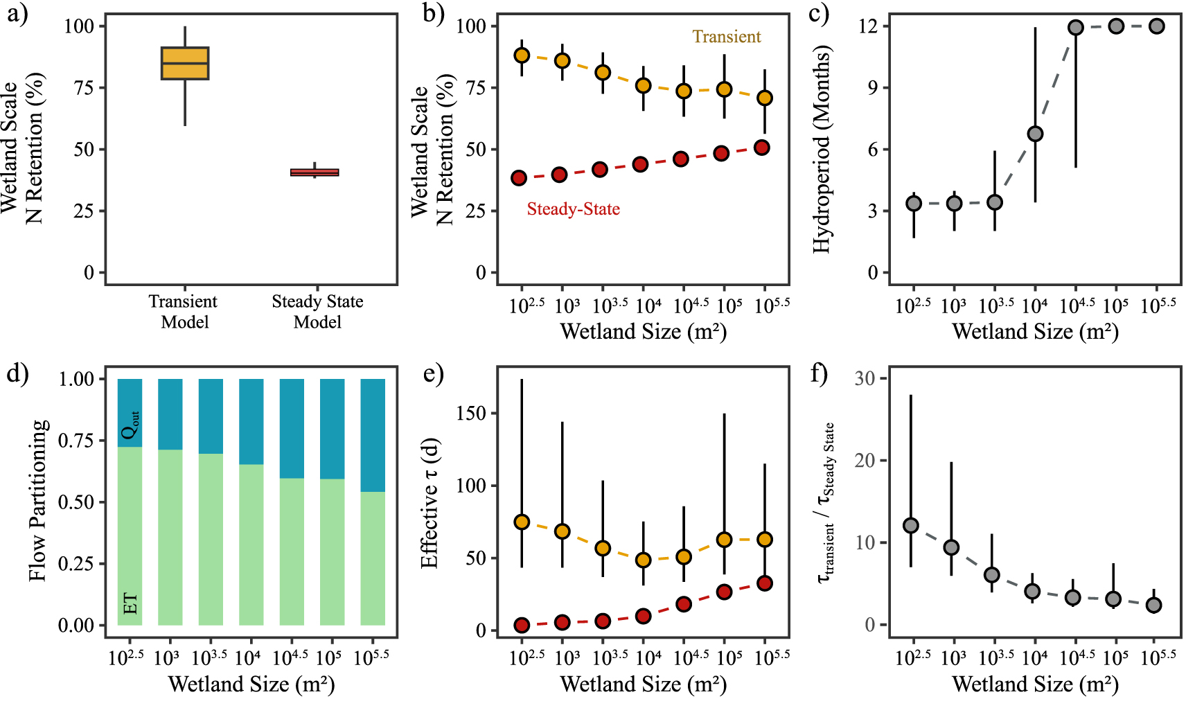
We first explored the behavior of prairie pothole wetlands in the North Dakota region to quantify how flow transience controls N retention. This was done by running the N retention model (equations (1)–(3)) for each of the 2395 wetlands over the 30 year timeframe (1985–2015). There were some years within this timeframe when data was not available for some wetlands, possibly due to drier conditions and detection limits, and this led to 12 570 wetland-years of simulation (table 1). A median N retention efficiency of 84% (interquartile range IQR: 79%–91%) was observed across these 12 570 wetland-years, in contrast to the steady state scenario where only 40% (IQR: 39%–42%) of the N entering the wetland was retained (figure 2(a)). For the steady state scenario, a single N retention efficiency was calculated for each of the 2395 wetlands, as a function of their size (equation 4). The range of retention efficiencies for the transient scenario was greater than the steady scenario, given it explicitly considered that retention efficiencies of a single wetland can vary across years, as a function of transient hydrology.
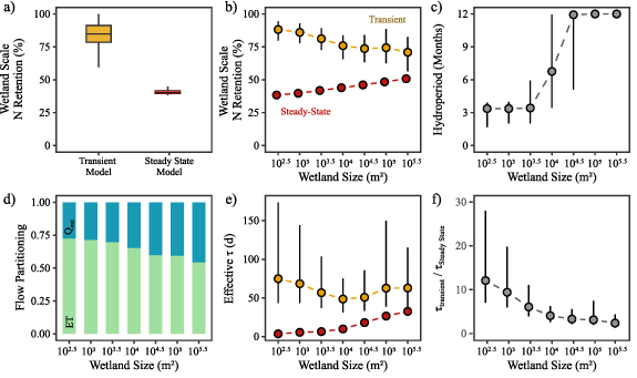
Figure 2. Size dependent relationships of wetland behavior in North Dakota. (a) Percent N retention of all GIWs in landscape for the steady state versus the transient model; (b) percent N retention of GIWs grouped by size. Differences in N retention were driven by differences in hydrologic behavior, and summarized in the following metrics: (c) hydroperiod; (d) flow partitioning of hydrologic inputs (P and Qin) leaving wetland as lateral outflows (Qout; blue bars) and ET (green bars); (e) effective residence time (τ) for the steady state and transient scenarios; (f) ratio of modeled transient residence time (τTS) to steady state residence time (τSS). The box extent and horizontal lines in (a) show the interquartile range and median, with the whisker showing the maximum/minimum values. The bounds in (b) to (f) show the interquartile range and the inner point is the median value of the results.
Download figure:
Standard image High-resolution imageWhen disaggregated by size, we found N retention to increase with wetland size under the steady state scenario, from 38% for small wetlands (102.5–103 m2) to 50% for large wetlands (105.5–106 m2). Interestingly, the relationship between N retention and size is reversed under the transient scenario, with greater N retention (88%) in the smaller wetlands compared to the larger ones (71%) (figure 2(b)). We hypothesize that this dependence of N retention on size and flow transience can be attributed to differences in flow dynamics between the small and large wetlands.
To explore this hypothesis further, we first studied the hydrologic dynamics of the wetlands. Small wetlands (<103.5 m2) in the prairie pothole region (PPR) have a median hydroperiod of four months (figure 2(c)), and typically fill up during the spring freshet and dry up over the summer months [30]. Such seasonal wetting-drying dynamics imply that a large proportion of water entering the wetland leaves as evapotranspiration. Our flow analysis highlights that in these small wetlands, only 28% of the water that comes in as snowmelt or runoff actually leaves as groundwater or surface water outflow, while the remaining 72% of water leaves as evapotranspiration (figure 2(d)). This is consistent with field studies in the PPR that have found that, in small wetlands, over 80% of the water can leave the system as ET, when considering losses in both the wetland and the surrounding uplands [30, 36]. Large wetlands (>104.5 m2), on the other hand, often have water for the entire year, and a greater proportion of incoming water leaves as lateral fluxes (43%) compared to ET based on our model results (figure 2(d)). The greater proportion of ET in small wetlands most likely contributes to a more terminal behavior for N retention in these small ephemeral systems.
Next, we compared the residence times and retention rate constants in small and large wetlands as a function of flow transience. For the steady state assumption, residence times increase as a function of wetland size [6], and the combined effect of a negative k–SA and a positive τ–SA relationship contributes to an increase in the N retention efficiency with increasing wetland size (figure 2(e)).
Transient systems are more complicated since a large proportion of the water entering the system might only leave the system through evapotranspiration, while the N is retained within the system—leading to different residence times for water and nitrogen. We estimated an effective nitrogen residence time (figure 2(e)) for the transient scenario by using the transient N retention efficiency (RTS) (figure 2(b)) and median k to solve for τTS using equation (4). We found that the effective residence time in the transient scenario to be greater than the steady state scenario, and the τ–SA relationship shows a unique U-shaped behavior, with the smallest and largest wetlands having the largest residence times (figure 2(e)). While residence times in larger wetlands are larger because of their larger volume to lateral flow ratio, residence times in smaller wetlands are larger under the transient assumptions due to the terminal nature of their flow dynamics. Effective residence times in these small, ephemeral systems can be 10–20 times greater than under steady state assumption, while for the larger wetlands residence times are similar under transient and steady state conditions (figure 2(f)).
3.2. Effect of climate variability and inundation dynamics on N retention
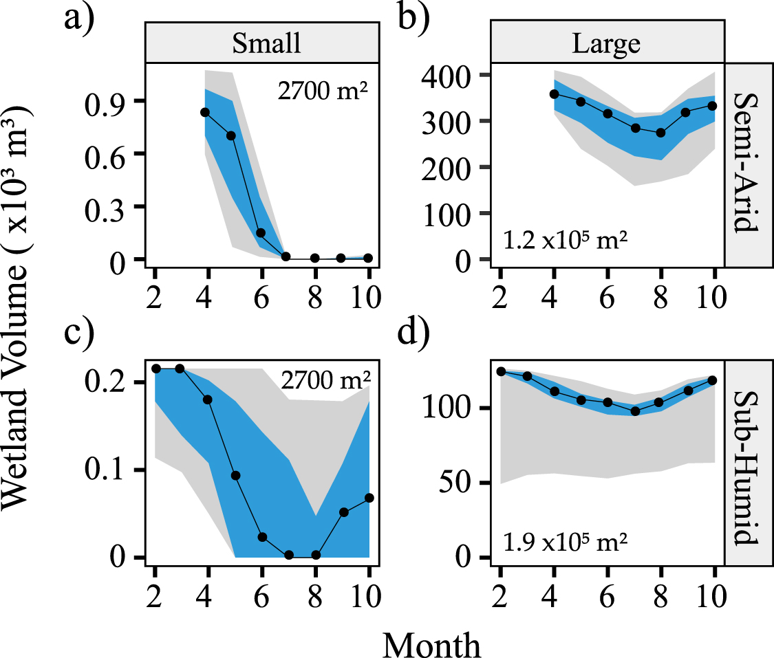
To further explore the impact of hydroclimatic variability on wetland N retention, we expanded the analysis from North Dakota to seven other wetlandscapes across the US. We found wetland inundation dynamics to be strongly driven by climate and wetland size. In the semi-arid PPR of North Dakota (aridity index AI = PET/P = 2.31), wetlands are frozen during the winter months and have peak inundation levels in April (figures 3(a) and (b)). This behavior is typical of snowmelt driven systems like the basin wetlands of Minnesota, prairie potholes in North Dakota and Nebraska Sandhills [25]. The climate drivers are further modified by wetland size, where small wetlands in the PPR typically fill up during the spring snowmelt and dry up over the summer months (figure 3(a)) while large wetlands often lose only a smaller proportion of their total volume during summer and rarely completely dry up (figure 3(b)). This contrasts wetlands in the more rainfed, humid systems like the pocosins in North Carolina (AI = 1.23), which have water for most of the year in both small and large wetlands, albeit the smaller wetlands have a greater drawdown magnitude compared to its volume (figures 3(c) and (d)).
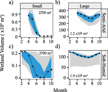
Figure 3. Monthly inundation volumes (regime curves) for example small and large wetlands in different climates. The black lines are median volumes for a small (102.5–103 m2) and large (105–105.5 m2) wetland in North Dakota (Semi-Arid; (a) and (b)) and North Carolina (Sub-humid; (c) and (d)), the blue bands show the 25th–75th percentile, and the gray band shows the 5th–95th percentile. The maximum area of the individual wetlands is indicated in the figure.
Download figure:
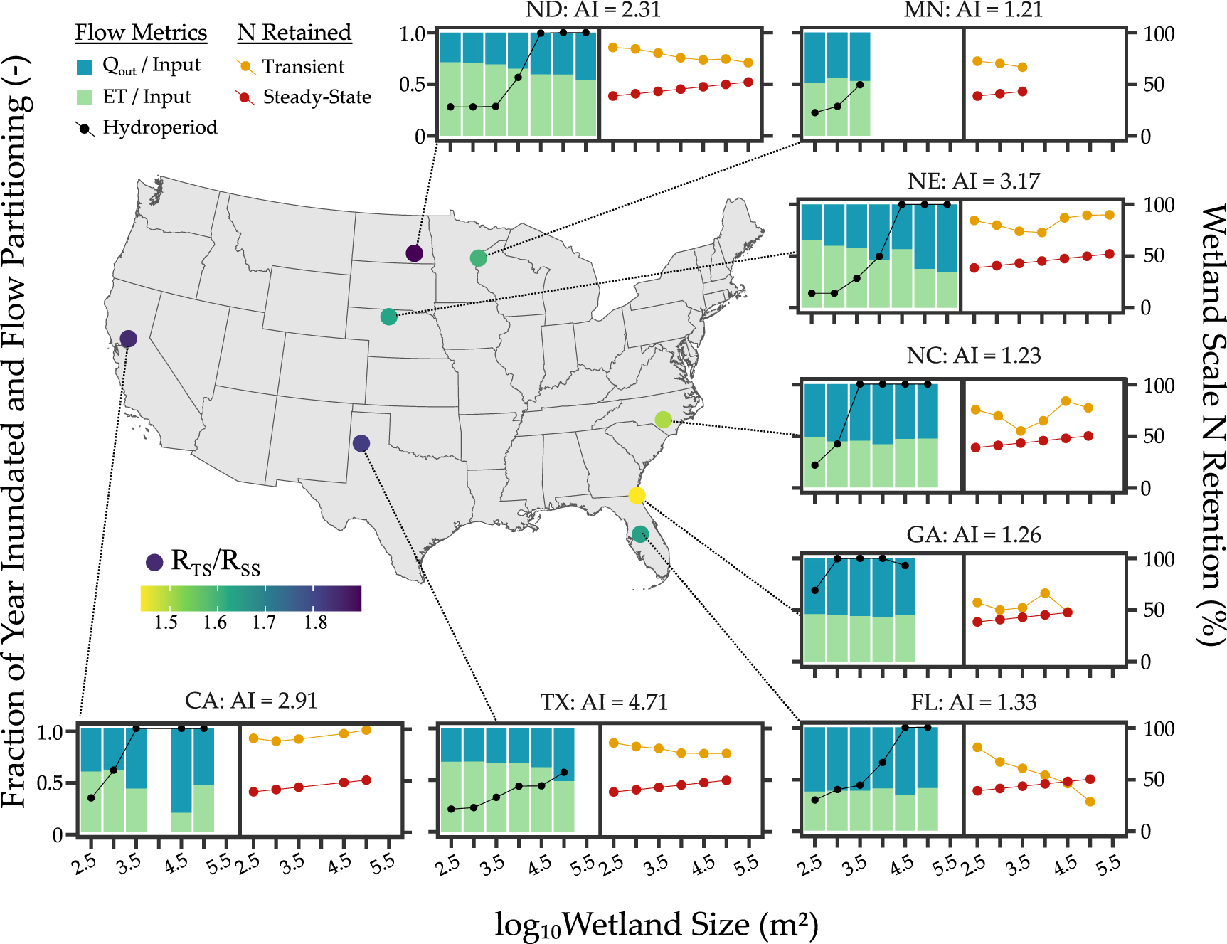
Standard image High-resolution imageThis pattern is consistent across the hydroperiods in all eight wetlandscapes (black lines in figure 4), with smaller wetlands in semi-arid landscapes (regions with AI >2, i.e. TX, NE, CA, ND) being more ephemeral (shorter hydroperiods), while humid landscapes have a greater proportion of more permanent wetlands. For example, the median hydroperiod for the largest size class (105–105.5 m2) in the Texas playas (AI = 4.71) is 6.8 months, while for the more humid North Carolina wetlands (AI = 1.23), the median hydroperiods for all wetlands >103.5 m2 is one year, indicating that a greater proportion of the wetlandscape is composed of more permanent wetlands.
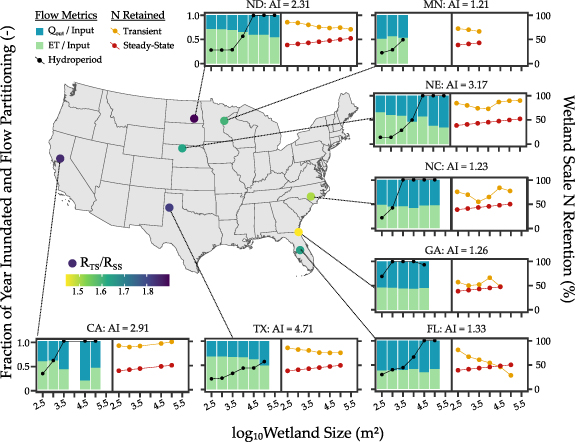
Figure 4. Hydrologic and N retention behavior across wetland sizes, and landscape regions. Differences in hydrologic behavior across wetland sizes and landscapes are apparent in the hydroperiod (black points) and flow partitioning (green and blue stacked bars). Water can leave the wetland as either lateral outflow (blue bars), or ET (green bars) and the relative proportion of these two fluxes is driven both wetland size, as well climate and geomorphology across various wetlandscapes. These differences in flow partitioning contribute to different patterns in transient N retention across wetlands (yellow points), with higher retention apparent in smaller wetlands in more arid landscapes (TX, ND) that have greater proportion of ET fluxes, and thus more terminal behavior. For all landscapes, the transient N retention is greater the steady state assumption (red points). Map inset shows the locations of the wetlandscapes, with the colored points indicating the ratio of the median transient and steady state N retention. Aridity index AI is defined here as PET/P.
Download figure:
Standard image High-resolution imageEvapotranspiration dominates the water partitioning in the semi-arid wetlandscapes (regions with AI >2, i.e. TX, NE, CA, ND), and typically accounts for greater than 50% of the incoming water (green bars in figure 4), with smaller wetlands having a greater proportion of ET fluxes. For example, ET loss accounted for 68% of the inflows in the small playas in Texas, but only 48% of the inflows for the larger playa wetland. More humid regions with aridity indices closer to 1 (FL, GA, NC, MN) have a greater proportion of lateral fluxes compared to ET, and no discernible flow partitioning differences with wetland size (figure 4). These wetlands may have extended periods when inflows to the wetland exceed evapotranspiration and allow for more continuous surface outflows regardless of wetland size.
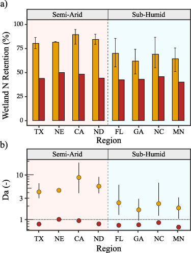
Finally, these hydrologic differences translate to different patterns of N retention. While for most wetlands, the transient assumption leads to greater N retention compared to the steady state assumption, the difference is greater for the semi-arid wetlandscapes, like the prairie potholes in North Dakota compared to the more humid wetlands in Georgia (figure 4). Overall, N retention percentages for the semi-arid systems are 1.63–1.82 times greater in the transient compared to the steady state scenario, while for the humid systems N retention is only 1.43–1.65 times greater in the transient scenario (figure 5(a)). Indeed, while the Damkohler number Da is greater than 1 for all regions in the transient cases (figure 5(b)), Da is consistently higher in the semi-arid systems. This suggests that the loss of N in the semi-arid wetlands are more driven by the biogeochemical processes rather than transport out of the system.
Figure 5. Regional estimates of N retention across different wetlandscapes. (a) Percent N retained in each wetlandscape. Transient flow assumptions (gold) lead to greater N retention more N than steady state assumptions (red). Bars show the median annual retention and bounds indicate the upper and lower quantiles. (b) Damkohler numbers of wetlands in each wetlandscape. Wetlands with Da <1 are considered to be transport dominated, and Da >1 to be dominated by biogeochemical processes.
Download figure:
Standard image High-resolution image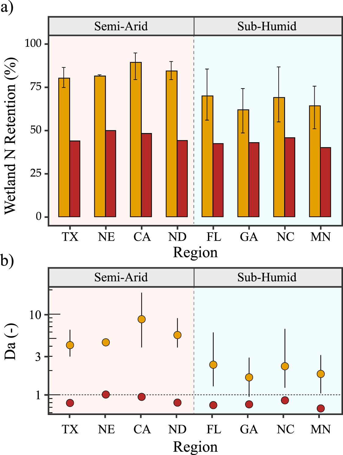
Of course, differences in the N retention patterns between wetlandscapes cannot be completely explained by aridity alone. For example, North Carolina and Florida wetlands have similar AI values, but different N retention dynamics (figure 4), and this can be attributed to differences in temporal patterns of rainfall, as well as differences in landscape attributes that drive N retention. While the patterns of N retention dynamics across humid and semi-arid systems is interesting, the exact magnitudes should be interpreted with caution, especially for regions with relatively few wetlands, making the size dependent patterns less reliable. Furthermore, it is important to note that the residence time estimation in the steady state scenario is based on an empirical relationship, and is thus invariant across the different wetlandscapes, while the transient scenarios are driven by the local inundation dynamics from remote sensing datasets. Despite these limitations, our analyses highlight that small, ephemeral wetlands have a greater potential to sequester nutrients and protect downstream waters, and this difference is more significant in semi-arid systems.
4. Summary and conclusions
The ability of wetlands to retain excess nutrients and protect downstream waters is a function of their hydrologic dynamics that drive nutrient inputs and biogeochemical factors that control processing rates. There is currently a lack of understanding on how temporal hydrologic dynamics drive nutrient retention patterns in wetlands across large spatial scales. Here, we develop a novel methodology to connect satellite-driven estimates of sub-annual wetland inundation dynamics to their nitrogen retention potential, across thousands of GIWs in eight US wetlandscapes. We show how small, ephemeral GIWs, especially in semi-arid landscapes, can be disconnected from their uplands for parts of the year due to high evapotranspiration rates, and this disconnectivity increases nitrogen retention. In semi-arid wetlandscapes such as the prairie potholes in North Dakota or the Texas playas, consideration of transient dynamics contributed up to 1.8 times increase in nutrient retention, while the increase was relatively smaller (∼1.5 times) in the more humid wetlands like the pocosins in North Carolina.
The study has a few key assumptions that should be addressed in future work. First, there are uncertainties in the remotely sensed GIW dataset [25] that arise from a combination of factors, including presence of clouds and canopy, coarse (once a month) temporal and spatial (30 m × 30 m) resolution of the data, inherent uncertainty in the GSW product, undefined dates of data capture to define the inundation pixels. However, despite these assumptions this dataset still provides the consistent national coverage of wetland inundation dynamics. Such uncertainties can be addressed in the future as new remotely sensed datasets of finer spatial and temporal resolution, such as Sentinel-2 [37], WorldView-3 [38], and those by commercial platforms such as Planet Lab (www.planet.com), are rapidly becoming available. The second major assumption arises from our description of the contributing areas, flow pathways and connectivity of the wetlands. We assumed a constant catchment to wetland area ratio, and an existing dataset for runoff estimation. This can be refined in future work using more accurate representation of contributing areas and partitioning of flows between surface and subsurface pathways as a function of landscape-specific geology. Finally, we assumed N concentrations entering the wetlands to be temporally invariant. Future work should explore how variability in the relationships between Cin and the flow Q can alter N retention [39].
Despite these challenges, this study, for the first time, develops a methodology to translate seasonality in GIW inundation dynamics to their role in N retention at the landscape scale. The study has a few key novel aspects—from a methodological perspective, it lays a new framework for wetland functional modeling by using, for the first time, temporally varying remote sensing data across thousands of wetlands to quantify their nutrient retention dynamics. As such datasets are becoming more common, future research can refine such methodologies and provide more validation using site specific datasets. From a fundamental science perspective, our modeling exercise highlights the sensitivity of N retention services of wetlands across a range of transient and steady state conditions, and allows us to differentiate retention between years and regions. Finally, from a wetland management perspective our work highlights how the disconnectivity of the wetlands is critical to maintain the integrity of downstream waters—the steady state assumption captures the behavior of a wetland with a constant, continuous connection to downstream waters, while the transient assumption highlights the potential for intermittent connections to downstream waters that is characteristic of less modified landscapes, and this disconnectivity increases the N retention potential, especially for the smaller, ephemeral wetlands.
Acknowledgments
Work conducted by F Y C and N B B is part of the project titled “Lake Futures” funded by the Global Water Futures program, Canada First Research Excellence Fund. Additional information is available at www.globalwaterfutures.ca. Additional financial support was provided by the National Science Foundation (OIA-2019561) for M K and J P.
Data availability statement
The data that support the findings of this study are available upon reasonable request from the authors.
Conflict of interest
Authors declare no competing interests.
- The University of Liverpool
- City University of Hong Kong (CITYU): Department of Physics
- Lawrence Livermore National Laboratory