

Retrieving gap-free daily root zone soil moisture using surface flux equilibrium theory
Published 17 September 2021 •
© 2021 The Author(s). Published by IOP Publishing Ltd
,
,
Citation Pushpendra Raghav and Mukesh Kumar 2021 Environ. Res. Lett. 16 104007DOI 10.1088/1748-9326/ac2441
You need an eReader or compatible software to experience the benefits of the ePub3 file format.
Article metrics
3497 Total downloads
0 Video abstract views
Submit
Submit to this JournalDates
- Received 4 February 2021
- Accepted 7 September 2021
- Published 17 September 2021

Peer review information
Method: Double Anonymous
Revisions: 2
Screened for originality? No
Abstract
Root zone soil moisture (RZSM) is a dominant control on crop productivity, land-atmosphere feedbacks, and the hydrologic response of watersheds. Despite its importance, obtaining gap-free daily moisture data remains challenging. For example, remote sensing-based soil moisture products often have gaps arising from limits posed by the presence of clouds and satellite revisit period. Here, we retrieve a proxy of daily RZSM using the actual evapotranspiration (ETa) estimates from Surface Flux Equilibrium Theory (SFET). Our method is calibration-less, parsimonious, and only needs widely available meteorological data and standard land-surface parameters. Evaluation of the retrievals at Oklahoma Mesonet sites shows that our method, overall, matches or outperforms widely available RZSM estimates from three markedly different approaches, viz. remote sensing data based Atmosphere-Land EXchange Inversion (ALEXI) model, the Variable Infiltration Capacity (VIC) model, and the Soil Moisture Active Passive (SMAP) mission RZSM data product. When compared with in-situ observations, unbiased root mean square difference of retrieved RZSM were 0.03 (m3 m−3), 0.06 (m3 m−3), and 0.05 (m3 m−3) for our method, the ALEXI model, and the VIC model, respectively. Better performance of our method is attributed to the use of both SFET for the estimation of ETa and non-parametric kernel-based method used to relate the RZSM with ETa. RZSM from our method may serve as a more accurate and temporally-complete alternative for a variety of applications including mapping of agricultural droughts, assimilation of RZSM for hydrometeorological forecasting, and design of optimal irrigation schedules.

Original content from this work may be used under the terms of the Creative Commons Attribution 4.0 license. Any further distribution of this work must maintain attribution to the author(s) and the title of the work, journal citation and DOI.
1. Introduction
Root zone soil moisture (RZSM) plays a critical role in the regional and global water cycle. The distribution of RZSM influences the incidence and intensity of floods (Norbiato et al 2008, Chen et al 2015), and droughts (Wang et al 2011, Samaniego et al 2018), mediates water quality (Zi et al 2016, Guo et al 2019), and has a range of ecohydrological implications including on crop productivity (Bolten et al 2009, Ines et al 2013, Chakrabarti et al 2014) and the growth and sustainability of trees (Porporato et al 2002, Anderegg et al 2015, Liu et al 2017). RZSM also plays a vital role in the partitioning of water and energy fluxes between land and atmosphere (Mintz and Serafini 1992, Lettenmaier and Famiglietti 2006, Trenberth et al 2007, Seneviratne et al 2010, Liu et al 2020). Despite its influence on a range of ecohydrological and atmospheric processes, observed RZSM data at daily interval is not readily available over large domains. Estimates of RZSM are often obtained through application of land surface models (LSMs) (Manabe 1969, Pan and Mahrt 1987, Xue et al 1991, Schaake et al 1996). These models, however, need extensive parameterization which continues to pose challenge in their application in data scarce environments, and oftentimes limits their accuracy (Xie et al 2007, Godfrey and Stensrud 2008, Veldkamp et al 2018). Recent efforts have incorporated remote sensing derived surface soil moisture for model-based predictions of RZSM (Manfreda et al 2014, Baldwin et al 2017, 2019, Reichle et al 2017). These methods also require fine spatial resolution data of soil properties at the least. Oftentimes, they require a full-on land surface parameterization. In addition, the remote sensing derived surface soil moisture products that may be used in these methods, e.g. by (Chauhan et al 2003, Njoku et al 2003, Entekhabi et al 2010, Kerr et al 2010, Torres et al 2012, Wagner et al 2013), often suffer from temporal and spatial data gaps due to presence of cloud cover, narrow swath, and sparse revisit schedules (Walker and Houser 2004, Sabaghy et al 2018, Mao et al 2019). For example, the temporal resolution of the latest 3 km SM product from the National Aeronautics and Space Administration Soil Moisture Active Passive (SMAP) mission, the SMAP/Sentinel-1 L2_SM_SP SM product (Das et al 2018) is reported to vary between 3 and 12 days depending on the revisit schedules of backscatter measurements of Sentinel-1A and Sentinel-1B sensors (Entekhabi et al 2010, Das et al 2016, Mao et al 2019). The percentage of missing days for SMAP L3 Radiometer Global Daily 36 km EASE-Grid Soil Moisture Version 6 (SPL3SMP) product and SMAP Enhanced L3 Radiometer Global Daily 9 km EASE-Grid Soil Moisture Version 3 (SPL3SMP_E) product at Oklahoma Mesonet sites, the study area under consideration, are over 50% for ascending and descending overpass and over 15% for composite data during 2015–2019 (see figure S1 in supporting information (available online at stacks.iop.org/ERL/16/104007/mmedia)). Another promising approach for estimating RZSM is based on the use of Atmosphere-Land EXchange Inversion (ALEXI) surface energy balance model (Anderson et al 1997, Mecikalski et al 1999, Anderson et al 2011), which to a large extent reduces the need for model calibration. ALEXI is a state-of-the-science tool that has been frequently used to track soil moisture stress in crops and forests (Anderson et al 2007a, 2007b, 2016b, Mishra et al 2013, Knipper et al 2019) and forms the basis for next generation of moisture stress measurements (Anderson et al 2016a, Guan et al 2017, Cawse-Nicholson et al 2020, Fisher et al 2020). However, Anderson et al (2007a) reported that good quality thermal infrared (TIR) imagery, which is often used for moisture retrieval over the continental US, was only available around 30% of the time in their study area.
Here, we propose a method based on the surface flux equilibrium theory (SFET) to retrieve fraction of available water ( ), a proxy for root-zone soil moisture. The proxy is then used to also obtain volumetric soil moisture (VSM) in the root zone using data of soil properties. The method yields gap-free daily estimate of
  , while only needing widely available meteorological data and standard land-surface parameters. The remainder of this paper is organized as follows: section 2 presents details of our methodology and a concise overview of the study area and datasets. Results are presented in section 3. Section 4 presents conclusions and related discussion.
2. Methods
2.1. SFET
McColl et al (2019) presented SFET where it was hypothesized that in the regions with no or minimal advective moisture convergence (e.g. inland continental regions), the near-surface atmosphere is in the state of ‘surface flux equilibrium’, i.e. the surface heating and surface moistening terms in the near-surface relative humidity budget are in the state of equilibrium at daily to monthly time scale. McColl and Rigden (2020) provided physical explanations for why the hypothesis stands using a simple model of an idealized atmospheric boundary layer. The approach does not require an explicit parameterization of land surface conditions as it assumes that the turbulent fluxes at the land surface (latent and sensible heat fluxes) are encoded in the near-surface atmospheric states (near surface air temperature and specific humidity, respectively). Using this theory, the Bowen ratio ( ) for a given location can be estimated as:
where  is Bowen ratio (
 ) [-], H is the sensible heat flux (W m−2),
  is the latent heat of vaporization (J kg−1),
  is the latent heat flux (W m−2),
  is the gas constant for water vapor (J kg−1 K−1),
  is the specific heat capacity of dry air at constant pressure (J kg−1 K−1),
  is the screen-level air temperature (K), and
  is the screen-level specific humidity of the air (kg kg−1). The latent heat flux (
 ) can then be obtained using the following relation derived based on surface energy balance:
where  is the net solar radiation (W m−2), and
  is the ground heat flux (W m−2). More details regarding the calculation of
  and
and  are provided in supporting information text S1. SFET based estimates of evapotranspiration have been shown to be remarkably accurate, with prediction errors comparable to errors in the eddy covariance measurements (McColl and Rigden 2020).
2.2. Soil moisture proxy retrieval
Here we retrieve fraction of available water ( ), a commonly used proxy for soil moisture (Anderson et al
2007a, Hain et al
2009, 2011).
), a commonly used proxy for soil moisture (Anderson et al
2007a, Hain et al
2009, 2011).  is defined as:
where  is the soil moisture content in the root zone soil layer (m3 m−3),
  is the soil moisture content at wilting point (m3 m−3),
  is the soil moisture content at field capacity (m3 m−3), and d is the root-zone depth (m). As latent heat flux is dominantly controlled by evapotranspiration of soil moisture, or its proxy, e.g.
  , can be potentially retrieved based on evapotranspiration estimates. For example, LSMs (Wigmosta et al
1994, Wood and Lettenmaier 1996, Panday and Huyakorn 2004, Hanasaki et al
2013, Wang et al
2013, Camporese et al
2014, Ferguson et al
2016) often use a simple soil moisture stress function to relate the simulated available water fraction (
, can be potentially retrieved based on evapotranspiration estimates. For example, LSMs (Wigmosta et al
1994, Wood and Lettenmaier 1996, Panday and Huyakorn 2004, Hanasaki et al
2013, Wang et al
2013, Camporese et al
2014, Ferguson et al
2016) often use a simple soil moisture stress function to relate the simulated available water fraction ( ) to the ratio of actual evapotranspiration (Eta) and potential evapotranspiration. This ratio, hereafter referred to as the fraction of potential evapotranspiration (
 , is defined as:
where  is actual evapotranspiration (mm d−1), and
  is potential evapotranspiration (mm d−1). Our method obtains
  using SFET as described in the previous section. The PET is estimated using the Penman–Monteith equation (Penman 1948, Monteith 1965) assuming the soil moisture conditions are at field capacity (see equation (3) in supporting information text S2). Once
  is evaluated, the underlying relation between
  and
and  is used to retrieve
  .
.
The relation between  and
and  is usually derived using pre-defined functions (Mahrt and Pan 1984, Wetzel and Chang 1987, Stewart and Verma 1992, Anderson et al
2007a, Hain et al
2009). By intercomparing four different functions that relate
is usually derived using pre-defined functions (Mahrt and Pan 1984, Wetzel and Chang 1987, Stewart and Verma 1992, Anderson et al
2007a, Hain et al
2009). By intercomparing four different functions that relate  and
and  , Hain et al (2009) reported better estimates of
  when it is derived as a nonlinear function of
  and
and  .
.  is the plant factor that captures the effects of stomatal control on the plant transpiration under well-watered conditions (see equation (7) in supporting information text S2). Instead of using a pre-defined function structure (for which the results are shown in figure S2 in supporting information), here we fit a single statistical relation between observed
  and
and  over all sites using a nonparametric kernel-based regression method (Nadaraya 1964, 1965, Watson 1964). The data used for developing the regression relation is restricted to a training period, and excludes the model evaluation period (more details are in section 2.4). Development of the relation using regional data is expected to moderate the discrepancy between estimated
  and observed soil moisture, especially those arising from the mismatch in root zone depth (for which
  is estimated) and the depth to which soil moisture observations are averaged to obtain
  for the training period. The kernel regression method (see equation (9) in supporting information text S2) has been demonstrated to successfully capture nonlinear relations effectively in numerous studies (Rubin et al
2010, Kannan and Ghosh 2013, Salvi and Ghosh 2013, Raghav et al
2020). Here, the predictors of the kernel regression are
for the training period. The kernel regression method (see equation (9) in supporting information text S2) has been demonstrated to successfully capture nonlinear relations effectively in numerous studies (Rubin et al
2010, Kannan and Ghosh 2013, Salvi and Ghosh 2013, Raghav et al
2020). Here, the predictors of the kernel regression are  and
and  , and the predictand is
  . The kernel regression algorithm described by Hayfield and Racine (2008) and implemented in the R-Package by (R Core Team 2013) is used. Notably, such a relation may be derived using any other observed soil moisture data sets existent within the region, such as SCAN and USCRN (Schaefer et al
2007, Diamond et al
2013). In regions where soil moisture data does not exist, as noted earlier,
. The kernel regression algorithm described by Hayfield and Racine (2008) and implemented in the R-Package by (R Core Team 2013) is used. Notably, such a relation may be derived using any other observed soil moisture data sets existent within the region, such as SCAN and USCRN (Schaefer et al
2007, Diamond et al
2013). In regions where soil moisture data does not exist, as noted earlier,  may be obtained using the pre-defined nonlinear functions.
2.3. Retrieving volumetric soil moisture ( )
)

 (derived in section 2.2) is converted to actual volumetric soil moisture (
 ,
,  ) using the field capacity (
 ) and wilting point (
 ) data using:

Here we assume the field capacity to be the volumetric water content at −33 kPa and wilting point to be the water content at −1500 kPa. In absence of site-specific root zone depth data,  and
and  used here are the average values within 0–100 cm from the soil surface.
2.4. Data used for model implementation, validation, and inter-comparison
The model is implemented in the state of Oklahoma and the results validated at the Oklahoma Mesonet sites (Brock et al
1995). Data from North American Land Data Assimilation System-Phase 2 (NLDAS-2) (Xia et al
2012a) such as air temperature, specific humidity, wind speed, shortwave downward radiation, longwave downward radiation, and near-surface atmospheric pressure are used to obtain estimates of potential evapotranspiration, ETa,  , and
, and  . The data has a temporal resolution of 1 h and spatial resolution of 1/8°, and so are the corresponding resolutions of our evapotranspiration estimates. Our method uses two vegetation dependent parameters viz., minimum solar radiation for transpiration (
 ), and a parameter related to vapor pressure deficit (
 ) for the calculation of PET (see equation (6) in supporting information S2). The model uses MODIS Global 500 m Collection 5 land cover (Friedl and Sulla-Menashe 2015) to obtain the most prevalent land cover by area within a NLDAS grid. Vegetation dependent land surface parameters corresponding to this land cover is assigned to the model grid based on the Noah model lookup table (Koren et al
2010). Notably, the model does not require any parameter calibration. Soil properties used for retrieving VSM are obtained from the MesoSoil database (Scott et al
2013), which includes physical properties of 13 soil types for 545 individual soil layers across 117 Oklahoma Mesonet sites. MesoSoil provides the data (e.g. sand-silt-clay fraction, volumetric water content at −33 kPa, −1500 kPa, residual and saturation water content, saturated hydraulic conductivity etc) at depths of 5 cm, 10 cm, 25 cm, 45 cm, 60 cm, and 75 cm.
) for the calculation of PET (see equation (6) in supporting information S2). The model uses MODIS Global 500 m Collection 5 land cover (Friedl and Sulla-Menashe 2015) to obtain the most prevalent land cover by area within a NLDAS grid. Vegetation dependent land surface parameters corresponding to this land cover is assigned to the model grid based on the Noah model lookup table (Koren et al
2010). Notably, the model does not require any parameter calibration. Soil properties used for retrieving VSM are obtained from the MesoSoil database (Scott et al
2013), which includes physical properties of 13 soil types for 545 individual soil layers across 117 Oklahoma Mesonet sites. MesoSoil provides the data (e.g. sand-silt-clay fraction, volumetric water content at −33 kPa, −1500 kPa, residual and saturation water content, saturated hydraulic conductivity etc) at depths of 5 cm, 10 cm, 25 cm, 45 cm, 60 cm, and 75 cm.
We validate the estimated  against the FWI measurements at the Oklahoma Mesonet sites (Brock et al
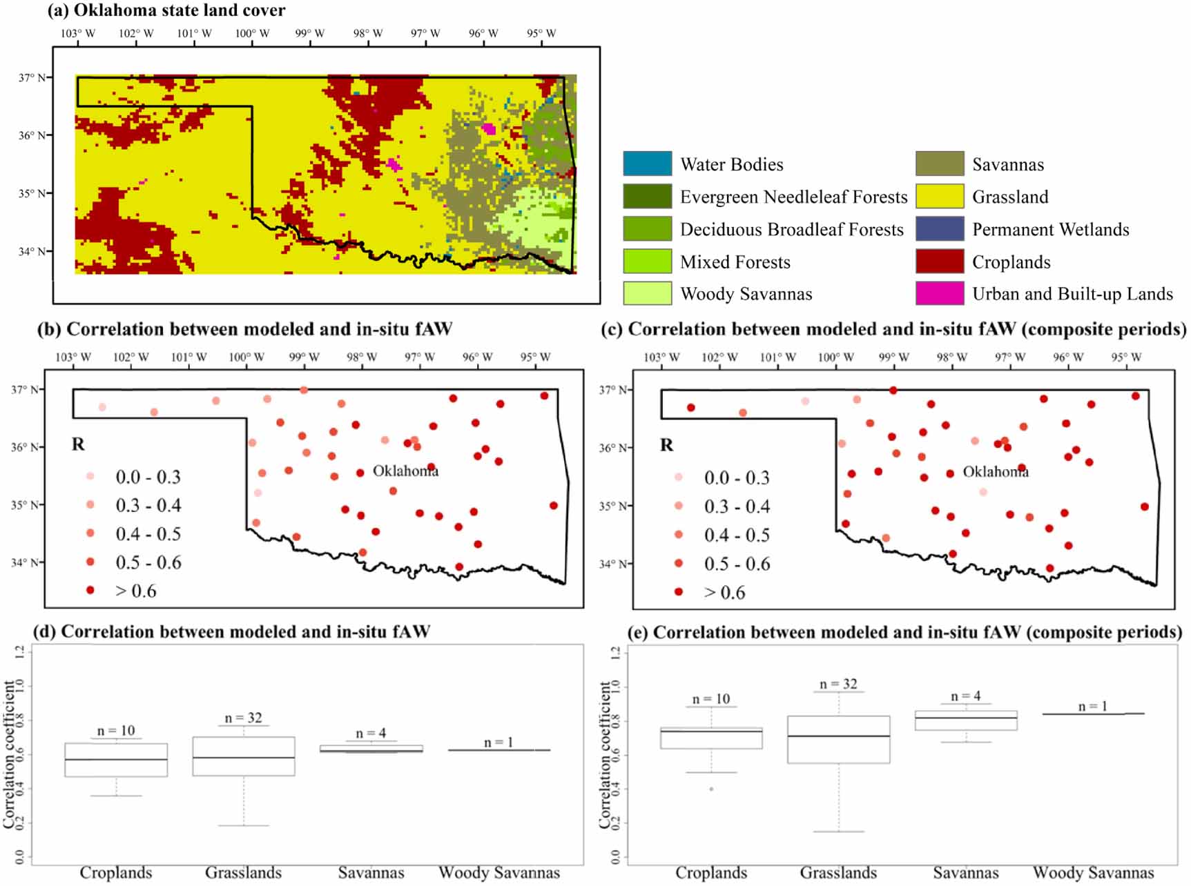
1995). The observation data network is located in the south-central region of the United States and spans entire Oklahoma with an area of ∼181 196 km2. Dominant land cover types include grassland (∼58%), croplands (∼15%), and forests with Savannas (∼15%), Woody Savannas (∼5%), and Deciduous Broadleaf Forests (∼3%) (see figure 2(a)). The network has at least one gauging station in each of Oklahoma’s 77 counties. The Mesonet network has been extensively used for validation of soil moisture or proxy products in previous studies (Drusch 2007, Gu et al
2008, Swenson et al
2008, Hain et al
2009, Fang et al
2013, Xia et al
2014). Notably, the Mesonet sites provide the opportunity for intercomparison not only with in situ data but also with retrievals from the ALEXI model (Anderson et al
1997, Mecikalski et al
1999, Anderson et al
2011).
against the FWI measurements at the Oklahoma Mesonet sites (Brock et al
1995). The observation data network is located in the south-central region of the United States and spans entire Oklahoma with an area of ∼181 196 km2. Dominant land cover types include grassland (∼58%), croplands (∼15%), and forests with Savannas (∼15%), Woody Savannas (∼5%), and Deciduous Broadleaf Forests (∼3%) (see figure 2(a)). The network has at least one gauging station in each of Oklahoma’s 77 counties. The Mesonet network has been extensively used for validation of soil moisture or proxy products in previous studies (Drusch 2007, Gu et al
2008, Swenson et al
2008, Hain et al
2009, Fang et al
2013, Xia et al
2014). Notably, the Mesonet sites provide the opportunity for intercomparison not only with in situ data but also with retrievals from the ALEXI model (Anderson et al
1997, Mecikalski et al
1999, Anderson et al
2011).
The validation is performed for the warm period (April–September) of 2002–2004. The period allows model evaluation against both in situ data and ALEXI model estimates. Figure S3 in supporting information shows the locations of stations at which we validated our model results. The selected sites cover a variety of land covers across Oklahoma (see figure 2(a)), and were also used in (Hain et al
2009) for evaluation of estimated  . For validation, estimated
  is compared against observed FWI. FWI has been demonstrated to be equivalent to observed
  at Mesonet sites with a correlation coefficient of 0.97 between computed
  and FWI (Hain et al
2009). Although FWI observations are available at fine temporal resolution (∼5 min) and at depths of 5 cm, 25 cm, 60 cm, and 75 cm (Illston et al
2008), due to the absence of site-specific root zone distribution data, the observations at all the sensor depths are averaged to obtain a depth-averaged FWI (Jackson et al
1996, Wagner et al
1999, Hain et al
2009). Days (∼ 17% of the total number of days during the warm period) with any missing value across depths were discarded in our comparisons. Notably, the nonparametric kernel regression that establishes a relation between
and FWI (Hain et al
2009). Although FWI observations are available at fine temporal resolution (∼5 min) and at depths of 5 cm, 25 cm, 60 cm, and 75 cm (Illston et al
2008), due to the absence of site-specific root zone distribution data, the observations at all the sensor depths are averaged to obtain a depth-averaged FWI (Jackson et al
1996, Wagner et al
1999, Hain et al
2009). Days (∼ 17% of the total number of days during the warm period) with any missing value across depths were discarded in our comparisons. Notably, the nonparametric kernel regression that establishes a relation between  and
and  (as outlined in section 2.2) is obtained using two years (2000–2001) of
  observation data and
  estimates at all the Mesonet sites used in this study. This training period for regression is mutually exclusive to the model validation period which ranges from 2002 to 2004. Derivation of a single regression relation that is then used for
  estimation at all the sites ensures the generality of the approach, as such a relation may be developed using any alternative soil moisture observation data as well.
Model results are also compared against other widely available temporally continuous root-zone soil moisture products. This includes variable infiltration capacity (VIC) model-based soil moisture product, that was generated in the NLDAS (Xia et al
2012b). The temporal resolution of the VIC simulated soil moisture within NLDAS is 1 h and its spatial resolution is 1/8°. We use VIC-simulated 0–100 cm soil moisture for the evaluation of our results. In addition, comparisons are also performed against the moisture proxy retrieval from the ALEXI model and the 9 km × 9 km SMAP L4 RZSM moisture product (Reichle et al
2017). As data of ALEXI moisture estimates are not available, the comparison is directly performed against the ALEXI model performance statistics reported in (Hain et al
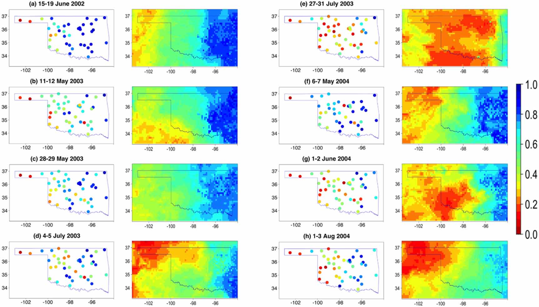
2009). In Hain et al (2009), the ALEXI model was executed at daily temporal resolution (but only on cloud-free days) and a spatial resolution of ∼10 km. For evaluation, moisture estimates were averaged over composite periods spanning 2–5 days each due to data coverage gaps caused by clouds. The composite periods included 15–19 Jun 2002, 11–12 May 2003, 28–29 May 2003, 4–5 Jul 2003, 27–31 Jul 2003, 6–7 May 2004, 1–2 Jun 2004, and 1–3 Aug 2004. Although we simulate gap-free daily  and VSM estimates and they are duly used for evaluation against in situ observations, composite estimates are obtained for intercomparison with ALEXI-derived
  estimates over the aforementioned composite periods. In contrast, as SMAP RZSM product is only available since March, 2015, comparison with it is performed for warm periods of 2015–2019.
Bias error (BE), mean absolute error (MAE), root mean square difference (RMSD), unbiased root mean square difference (ubRMSD), and Pearson correlation coefficient ( ) are used as performance metrics to assess the accuracy of
  estimates against in situ data. As the standard
  is sensitive to biases in the mean or high extreme values (outliers), here we also use the
  , a metric used by SMAP to quantify the product accuracy (Entekhabi et al
2010).
, a metric used by SMAP to quantify the product accuracy (Entekhabi et al
2010).
3. Results and explanations
3.1. Evaluation of temporal variations in simulated

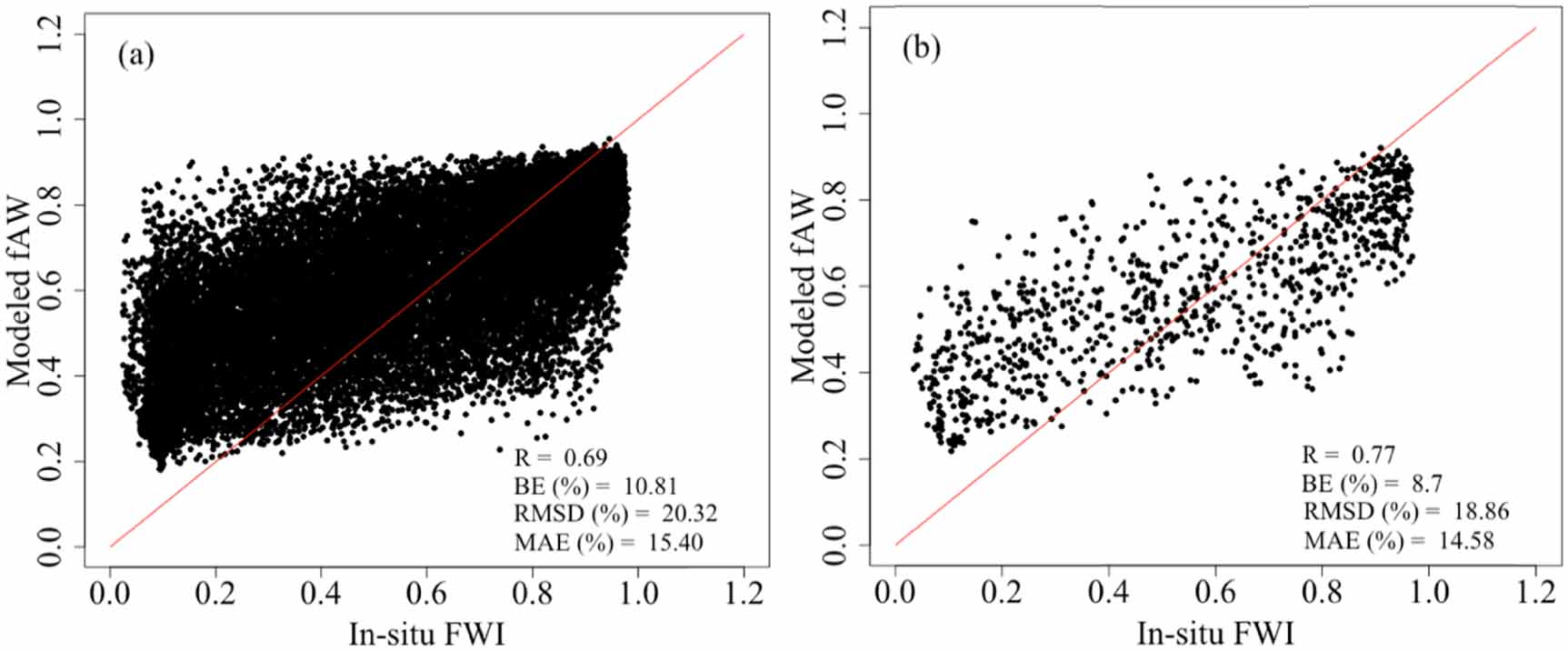
The retrieved  , using the method outlined in section 2, captures more than 48% (R = 0.69) of the variations in the observed FWI (see figure 1(a)). For the same eight composite periods as used in Hain et al (2009), the model’s performance is better during the composite periods (figure 1(b)) i.e. when clear sky conditions prevail, w.r.t. all periods (figure 1(a)). The possible reason for this is that the estimates of net radiation (and therefore latent heat flux) are generally more accurate during the largely clear sky, non-raining days. This is demonstrated at selected FluxNet sites where observed net short wave radiation data is available for evaluation (see figures S4 and S5 in supporting information). Overall, with respect to the observed, the presented method overestimates drier conditions and underestimates wetter conditions. This is in line with the conclusions in other studies (Allen et al
1998, Scott et al
2003, Akuraju et al
2017), where also it was observed that the relation between
, using the method outlined in section 2, captures more than 48% (R = 0.69) of the variations in the observed FWI (see figure 1(a)). For the same eight composite periods as used in Hain et al (2009), the model’s performance is better during the composite periods (figure 1(b)) i.e. when clear sky conditions prevail, w.r.t. all periods (figure 1(a)). The possible reason for this is that the estimates of net radiation (and therefore latent heat flux) are generally more accurate during the largely clear sky, non-raining days. This is demonstrated at selected FluxNet sites where observed net short wave radiation data is available for evaluation (see figures S4 and S5 in supporting information). Overall, with respect to the observed, the presented method overestimates drier conditions and underestimates wetter conditions. This is in line with the conclusions in other studies (Allen et al
1998, Scott et al
2003, Akuraju et al
2017), where also it was observed that the relation between  and
and  is ineffective when soil moisture conditions are above (below)
  (
( ).
).
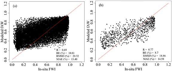
Figure 1. Comparison between daily observed and simulated fraction of available water ( ) at selected Oklahoma Mesonet stations (identified in figure S3 in supplement information) during April–September of 2002–2004. The red straight line is the 1:1 line. Figure (a) shows the comparison for all days during April–September, 2002–2004, (b) shows comparisons for the eight composite periods (see section 2.4 for definition of composite periods).
Download figure:
Standard image High-resolution imageComparison of our  estimates against those obtained from ALEXI for the composite periods shows that our method, overall, matches or outperforms the ALEXI results (as reported in table 2 of Hain et al (2009)) in the study area. ALEXI
  has a larger scatter with
  of 0.48 as compared to a
  of 0.60 or R of 0.77 (see figure 1(b) and table 1) from our method. Our method shows a slightly larger positive bias, with
  of 8.7% as compared to BE of −4.3% for ALEXI model. The RMSE and MAE are found to be 18.86% (21.3%) and 14.58% (17.7%) respectively for our method (ALEXI model). It is to be noted that Hain et al (2009) used a blended relation between
  and
and  but we use a nonparametric kernel-based method for the same. To assess if better performance of
  estimates from our method w.r.t. the ALEXI estimates is due to the use of SFET or the kernel-based method, we regenerate the
  estimates using the blended relation used in Hain et al (2009). Results (figures 1(b) and S2(b)) show our model performance (R = 0.77) does not change for the composite periods depending on the use of the nonparametric kernel-based method and the blended relation, and the estimates from either are better than that from ALEXI (R = 0.69, see table 1). Notably, the nonparametric kernel-based method yields better model performance when considering estimates from all the days (see figure 1(a) vs. figure S2(a)). These comparisons indicate better
  estimates from our method is a result of the use of both SFET to obtain evapotranspiration and the non-parametric kernel-based method used to obtain the relation between
  and
and  . Given that ALEXI derived
  estimates have been demonstrated to be more effective than Eta Data Assimilation System (EDAS) for accurate Numerical Weather Prediction (NWP) forecasts (Hain et al
2009), by extension, it may be claimed that estimates from our method will overperform the EDAS product as well. Notably, our method also provides temporally continuous daily estimates. In contrast, ALEXI estimates which uses TIR data suffer from large data gaps due to the presence of clouds and other satellite operational failures (Liou and Kar 2014).
estimates have been demonstrated to be more effective than Eta Data Assimilation System (EDAS) for accurate Numerical Weather Prediction (NWP) forecasts (Hain et al
2009), by extension, it may be claimed that estimates from our method will overperform the EDAS product as well. Notably, our method also provides temporally continuous daily estimates. In contrast, ALEXI estimates which uses TIR data suffer from large data gaps due to the presence of clouds and other satellite operational failures (Liou and Kar 2014).
Table 1. Error statistics for soil moisture proxy retrieved by our method and ALEXI during composite days at Mesonet stations. The error statistics for ALEXI shown here, have been obtained from Hain et al (2009).
| R | RMSD ( ) ) | BE ( ) ) | MAE ( ) ) | |
|---|---|---|---|---|
| Our method | 0.77 | 18.86 | 8.7 | 14.58 |
| ALEXI | 0.69 | 21.3 | −4.3 | 17.7 |
Table 2. Error statistics for volumetric soil moisture  retrieved by our method, ALEXI, and VIC model during composite days at Mesonet stations. The error statistics for ALEXI shown here, have been taken from Hain et al (2009).
RMSD 
| BE 
| MAE 
| ubRMSD 
| |
|---|---|---|---|---|
| Our method | 0.03 | −0.005 | 0.02 | 0.03 |
| ALEXI | 0.06 | −0.01 | 0.05 | 0.06 |
| VIC | 0.11 | 0.10 | 0.10 | 0.05 |
Figures 2(b) and (c) shows the spatial variation of temporal correlations between daily  estimates for April–September (composite periods) of 2002–2004 from our method and in-situ observations. The correlation is positive at all the sites with the highest correlation of 0.77 (0.99) and the lowest correlation of 0.18 (0.11) at 0.05 significant level (see figures 2(d) and (e)). Between different land covers, the highest correlation is found in Woodland Savanna while the lowest correlation is observed in cropland areas (see figure 2(d)). Relatively poor performance in croplands w.r.t. woodland is often attributed to the heterogeneity introduced by irrigation and is consistent with the conclusions of Naeimi et al (2009). Notably, the Bowen ratio obtained from SFET (see equation (1) that is then used here for evaluation of
  (using equations (4) and S9), is an integrated land-atmosphere feedback response of areas surrounding the Mesonet station. Hence,
  derived from this method is likely to represent an effective soil moisture within the grid (of spatial resolution 1/8°), and may diverge from point estimates especially if the area experiences significant moisture heterogeneity.
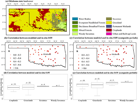
Figure 2. (a) MODIS Global 500 m Collection 5 land cover map of Oklahoma, (b) correlation between daily modeled  estimates and in-situ observations during warm periods of 2002–2004 at Oklahoma Mesonet sites, (c) correlation between modeled
  estimates and in-situ observations during the eight composite periods, (d) box plots of correlation coefficients shown in panel b for different land cover types, and (e) box plots of correlation coefficients shown in panel c for different land cover types. The dark black line in each boxplot shows the mean correlation for each land cover. The n-value at the top of each boxplot is the number of Mesonet sites within a particular land cover.
Download figure:
Standard image High-resolution image3.2. Evaluation of spatial variations in simulated

The retrieved  , overall, captures the spatial gradient of root-zone soil moisture conditions within the study area (figure 3). For example, for the composite period 15–19 June 2002, observed dry soil moisture conditions in extreme western Oklahoma and wet soil moisture conditions in eastern Oklahoma are reflected in the model estimates as well (see figure 3(a)). Similarly, our method also retrieves the dry soil moisture conditions all across Oklahoma during the composite period 27–31 July 2003 (figure 3(e)). Although, the overall spatial variability of soil moisture is captured by our model, there are disagreements. This could be due to a number of factors including scale mismatch between point measurements and our retrieval which is performed using meteorological data over a 0.125° × 0.125° grid. Additional sources of errors may be from varying
  vs.
vs.  relations across different land covers, quality of input data, and errors in estimate of ET especially on cloudy days.
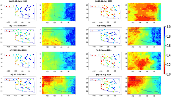
Figure 3. Spatial maps of  over the state of Oklahoma for different composite periods. For each composite period, the left panel shows in-situ observations of
  at different mesonet sites and the right panel shows retrieved
  using our method.
Download figure:
Standard image High-resolution imageNext, the average of daily spatial correlations for all days during April–September of 2002–2004 is obtained. The average spatial correlation using data from all aforementioned days is equal to 0.62 (see figure S6 in supplement information). The corresponding average correlation for the eight composite periods is 0.71. During the eight composite periods, the highest correlation is 0.84 for the composite period 15–19 June 2002 when the soil moisture conditions are wettest (see figure 3(a)) and the lowest correlation is 0.54 during the composite period 27–31 July 2003 when the moisture conditions are driest (see figure 3(e)). The difference in model performance between wet and dry dates is likely due to multiple factors, including the existence of a larger spatial gradient in soil moisture during the wet composite period, and a smaller sensitivity of moisture dynamics on evapotranspiration when the ground is dry.
3.3. Retrieving actual soil moisture
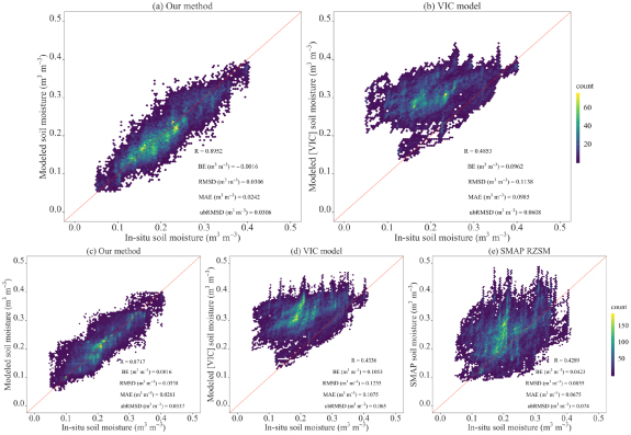
The retrieved  estimates are converted to VSM using the method outlined in section 2.3. A comparison between VSM estimates from our method and observations is performed (figure 4(a)). The correlation coefficient between the simulated daily soil moisture from our model and observed during the warm period of 2002–2004 is close to 0.90 when considering all the observation sites into the analysis. The significant increase in correlation for VSM w.r.t. that for
  (0.9 vs. 0.69 as seen in figures 4(a) and 1(a), respectively) is attributable to spatial heterogeneity in soil properties (see supplement figure S7). The model, overall, captures the temporal dynamics of VSM in diverse land cover types (figure S8 in supplementary information), although just like for
  (see figure 1) lower (higher) moisture values are overpredicted (underpredicted). We also compare VSM estimates from VIC model (figure 4(b)). In contrast to VSM estimates from our model, the VIC model estimates show a larger scatter with a R of 0.49. Furthermore, the VIC model overestimates the VSM observations with a bias error of 46.46% of the observations (see figure 4(b)). These results are consistent with Xia et al (2015) where it was reported that VIC model overestimated soil moisture. Overall, VSM estimates from our model (VIC model) show correlation, bias, RMSD, MAE, and unbiased RMSD of 0.90 (0.49), −0.78% (46.46%), 14.79% (54.95%), 11.71% (47.59%), and 0.03
  (0.06
(0.06  ), respectively. We also evaluate the error statistics for VSM retrievals during the eight composite periods (table 2). Results show our method outperformed both ALEXI and VIC model estimates. VIC model shows the largest bias errors among the three methods. Notably, our SM estimates adequately meet the SMAP mission requirement of
  to be less than
  (Chan et al
2016). Inter-comparison of RZSM estimates from the proposed method, VIC, and SMAP L4 RZSM product for warm periods of 2015–2019 further affirm the superior performance of the proposed method (see figures 4(c)–(e)) against these widely available sister products.
(Chan et al
2016). Inter-comparison of RZSM estimates from the proposed method, VIC, and SMAP L4 RZSM product for warm periods of 2015–2019 further affirm the superior performance of the proposed method (see figures 4(c)–(e)) against these widely available sister products.
Figure 4. Comparison between daily observed and simulated volumetric soil moisture at the Oklahoma Mesonet sites (shown in figure S3 of supplementary information). (a) SM estimates from our method, (b) SM estimates from the VIC model, (c) SM estimates from our method, (d) SM estimates from the VIC model, and (e) SM estimates from SMAP. Top panel shows the comparison during April–September of 2002–2004, the period for which performance statistics of ALEXI based estimate are also available thus allowing intercomparison with it. The bottom panel shows the comparison during April–September of 2015–2019 during which both SMAP RZSM and VIC model data are available. The red straight line is the 1:1 line.
Download figure:
Standard image High-resolution image
4. Conclusions and synthesis
This study presented a new method to obtain daily estimates of RZSM proxy and volumetric RZSM. The method was based on SFET, and only needs readily available meteorological data and standard land surface parameterizations to obtain estimates of moisture proxy. In other words, the method is ‘calibration-free’ and thus suitable for predictions in ungauged basins. Soil moisture proxy estimates from the method were in good agreement with the in-situ measurements at the Oklahoma Mesonet sites both temporally and spatially. The estimate of volumetric soil moisture in the root zone adequately met the SMAP soil moisture retrievals requirement of  .
.
An intercomparison of our estimate with the ALEXI model, which forms the basis for the next generation of moisture stress measurements (Anderson et al
2016a, Guan et al
2017, Cawse-Nicholson et al
2020, Fisher et al
2020), showed our method matched or outperformed ALEXI derived estimates. Better performance was found to be due to two reasons, a better evapotranspiration estimate using SFET and use of the non-parametric kernel-based method to obtain the relation between  and
and  . Another advantage of our method is its gap-free nature. In contrast, ALEXI or other TIR imagery-based retrievals of soil moisture provide estimates only during clear sky days as thermal imagery cannot be collected on cloudy days. Also, unlike our method, TIR-based methods for soil moisture proxy retrievals are dependent on a number of land surface parameters which are difficult to obtain in many cases. Given that ALEXI derived moisture proxy estimates have been demonstrated to be more effective than EDAS for accurate NWP forecasts (Hain et al
2009), by extension, it may be claimed that estimates from our method will overperform the EDAS product as well. Comparison against estimated moisture from VIC, a widely used land surface model, and SMAP L4 RZSM product which is generated by assimilating SMAP L-band brightness temperature observations into the NASA Catchment land surface model, showed our results outperformed them as well. These results indicate the advantage of our method over widely used land surface models, even while they use assimilation.
. Another advantage of our method is its gap-free nature. In contrast, ALEXI or other TIR imagery-based retrievals of soil moisture provide estimates only during clear sky days as thermal imagery cannot be collected on cloudy days. Also, unlike our method, TIR-based methods for soil moisture proxy retrievals are dependent on a number of land surface parameters which are difficult to obtain in many cases. Given that ALEXI derived moisture proxy estimates have been demonstrated to be more effective than EDAS for accurate NWP forecasts (Hain et al
2009), by extension, it may be claimed that estimates from our method will overperform the EDAS product as well. Comparison against estimated moisture from VIC, a widely used land surface model, and SMAP L4 RZSM product which is generated by assimilating SMAP L-band brightness temperature observations into the NASA Catchment land surface model, showed our results outperformed them as well. These results indicate the advantage of our method over widely used land surface models, even while they use assimilation.
Although our validation results showed an overall satisfactory performance, it is to be noted that the performance is not competent across all soil moisture states and land covers. Our method especially fell short to capture extreme dry soil moisture conditions. Also, the performance was relatively poor in cropland settings. Subpar performance on occasions can be from multiple sources including (a) scale mismatch between the point measurements and model pixel, (b) quality and resolution of input meteorological data, (c) heterogeneity in soil properties, especially when converting moisture proxy to volumetric moisture, (d) absence of strong relation between fractional moisture content and the ratio of actual to potential evapotranspiration for extremely wet and dry moisture states, (e) mismatch between the actual root zone depth and the depths to which moisture observations are available and/or averaged for comparison, and (f) violation of assumptions that are inherent in SFET. Despite these limitations, this study highlights the advantages of our method over remote-sensing retrievals and land surface model predictions for RZSM retrievals. These advantages make the presented method apt for continuous assimilation of moisture in land surface and numerical weather prediction models. Gap-free and calibration-free moisture estimates from this method can be useful for many applications such as tracking crop stress, monitoring agriculture drought, irrigation management, estimation of groundwater recharge, etc. Future efforts towards improving the retrieved moisture estimates from the method may focus on disaggregation of evapotranspiration and use of alternative meteorological forcing products. To further improve confidence in the applicability of the method for a wider range of settings, forthcoming studies may perform evaluation in other hydroclimatic regions.
Acknowledgments
This work is partially supported by NSF OIA-2019561, NSF EAR-1920425, and NSF EAR- 1856054. We thank Collin Mertz for providing the Oklahoma Mesonet soil moisture and soil properties data which were used for the validation of our results. All analyses were carried out in R www.r-project.org/ and for this, we are very much thankful to the R Core Team (2020).
Data availability statement
The Oklahoma Mesonet soil moisture data can be obtained upon reasonable request at www.mesonet.org/index.php/past_data/data_request_form. The native NLDAS-2 and SMAP data used in this study are available from the respective data repositories at https://disc.gsfc.nasa.gov/ and https://nsidc.org/data/smap/smap-data.html, respectively. Data that support the findings of this study will be made available upon reasonable requests to the authors.
The data that support the findings of this study are available upon reasonable request from the authors.
Code availability statement
Codes will be made available upon reasonable request from the authors.
Conflict of interest
Authors declare no competing interests.
- The University of Liverpool
- City University of Hong Kong (CITYU): Department of Physics
- Lawrence Livermore National Laboratory